Overview
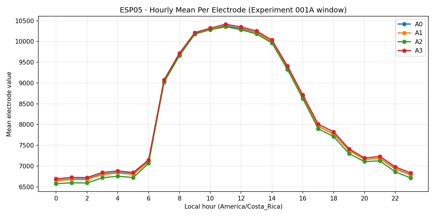
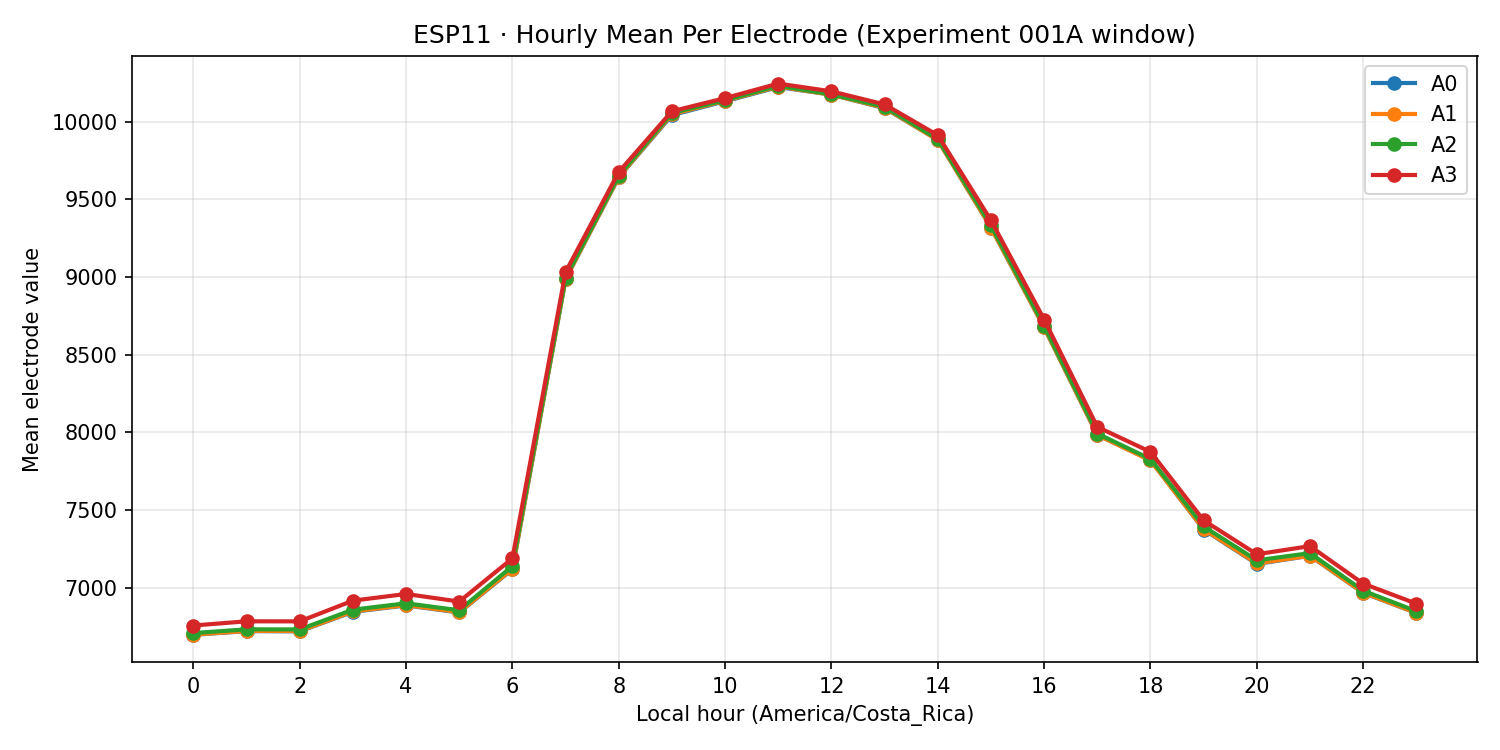
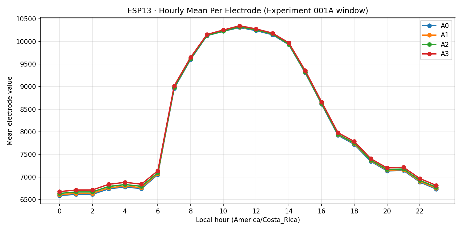
Motivation. Look inside the ESP averages: are the four electrodes tightly clustered (small spread) or sitting at different levels? If “state” can be sensed by any single electrode (against a common ground), we expect small spreads and phase‑coherent waveforms.
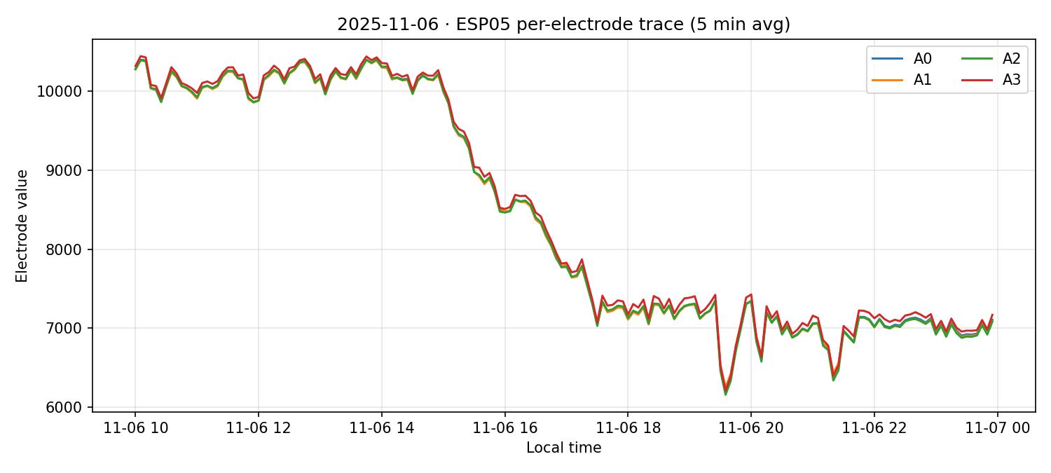
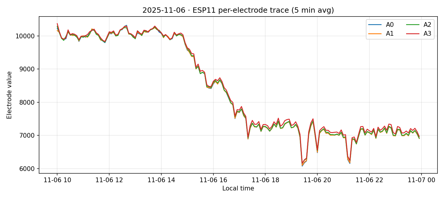
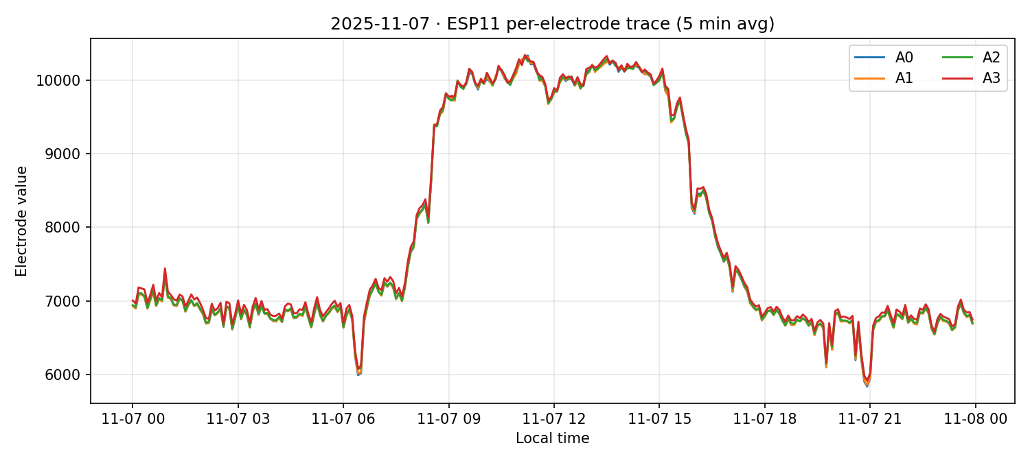
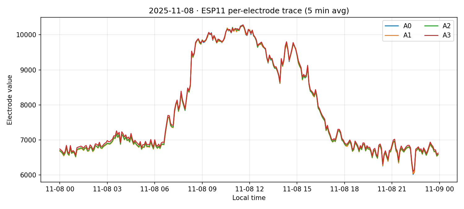
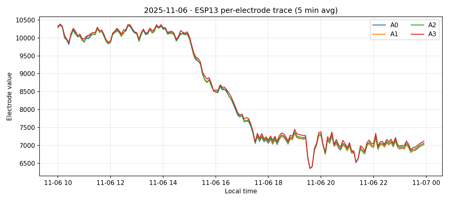
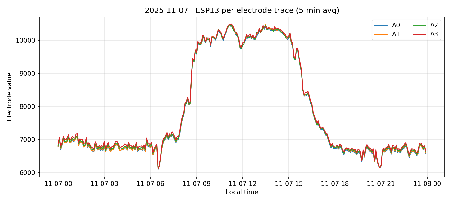
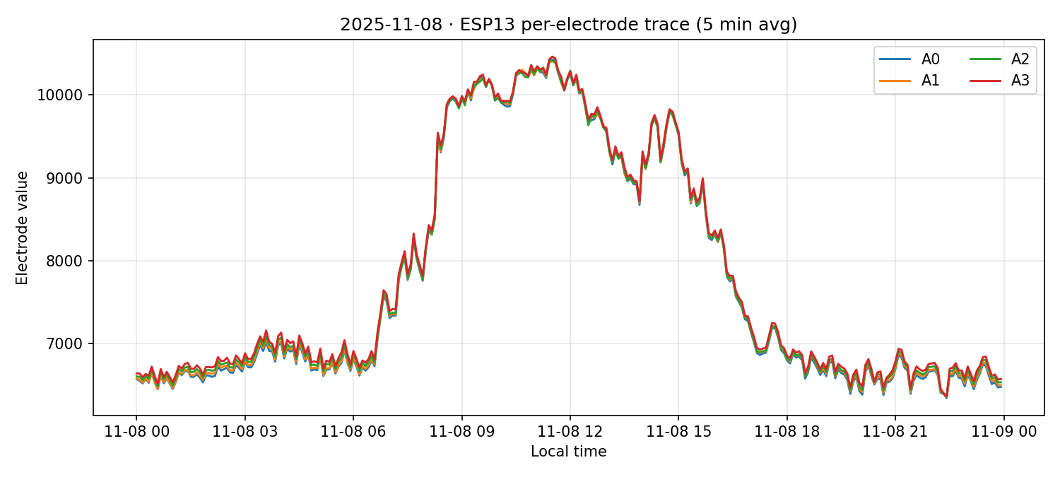
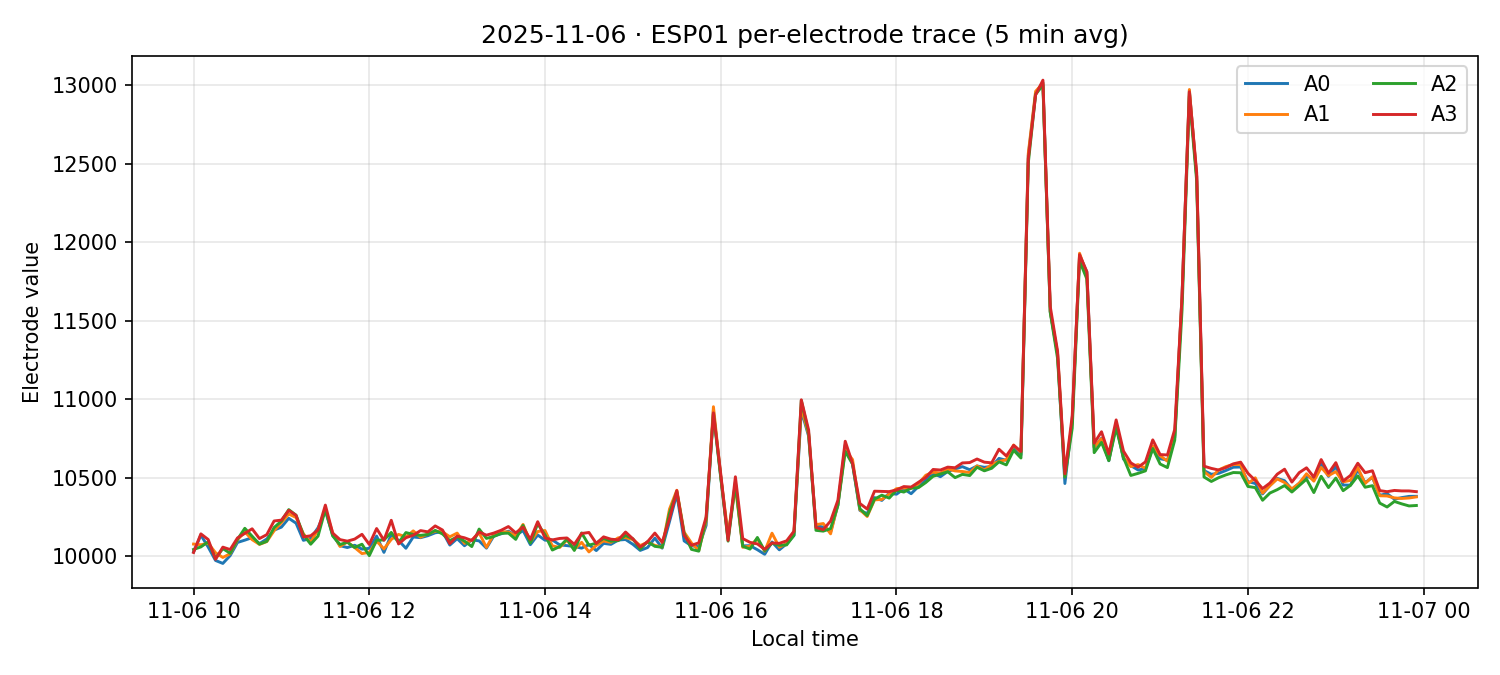
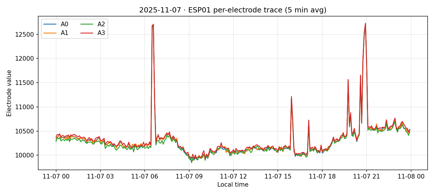
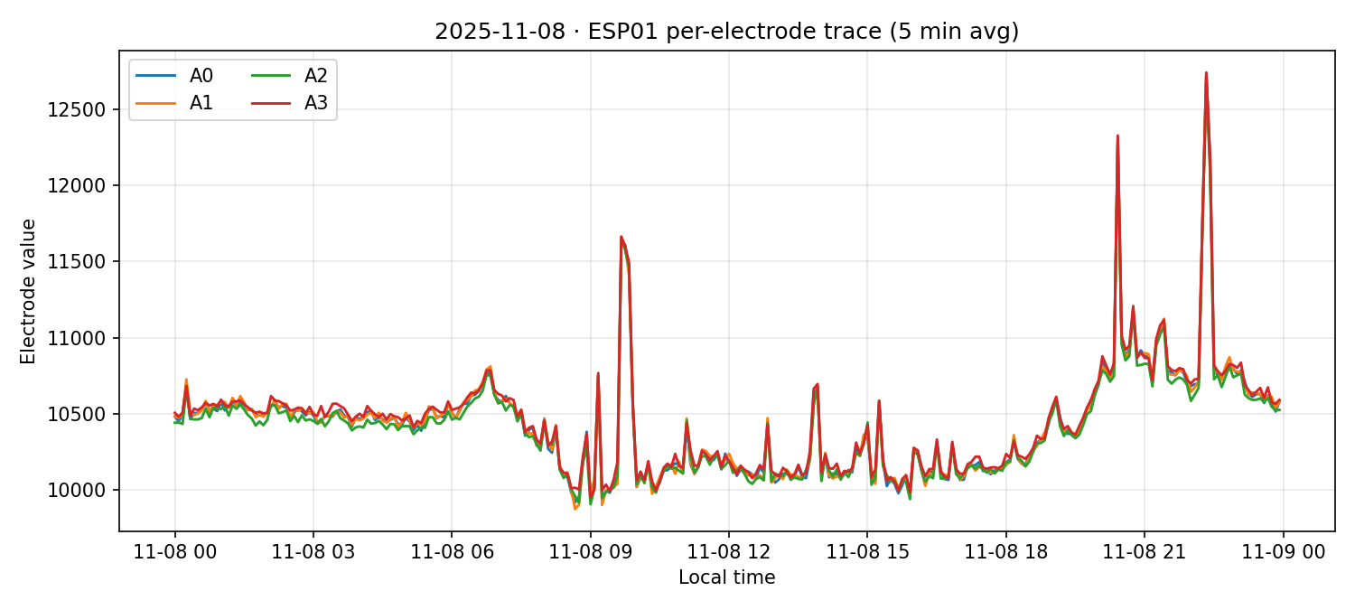
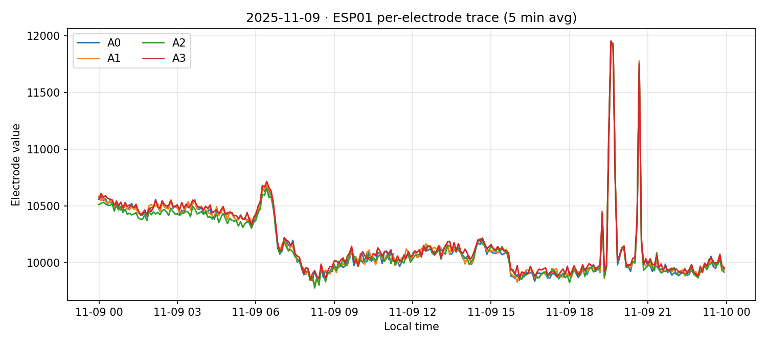
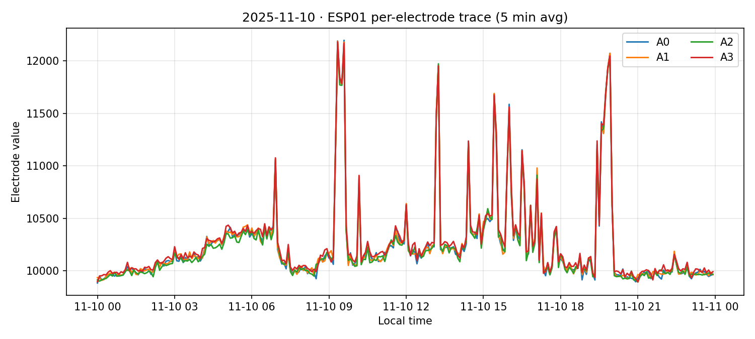
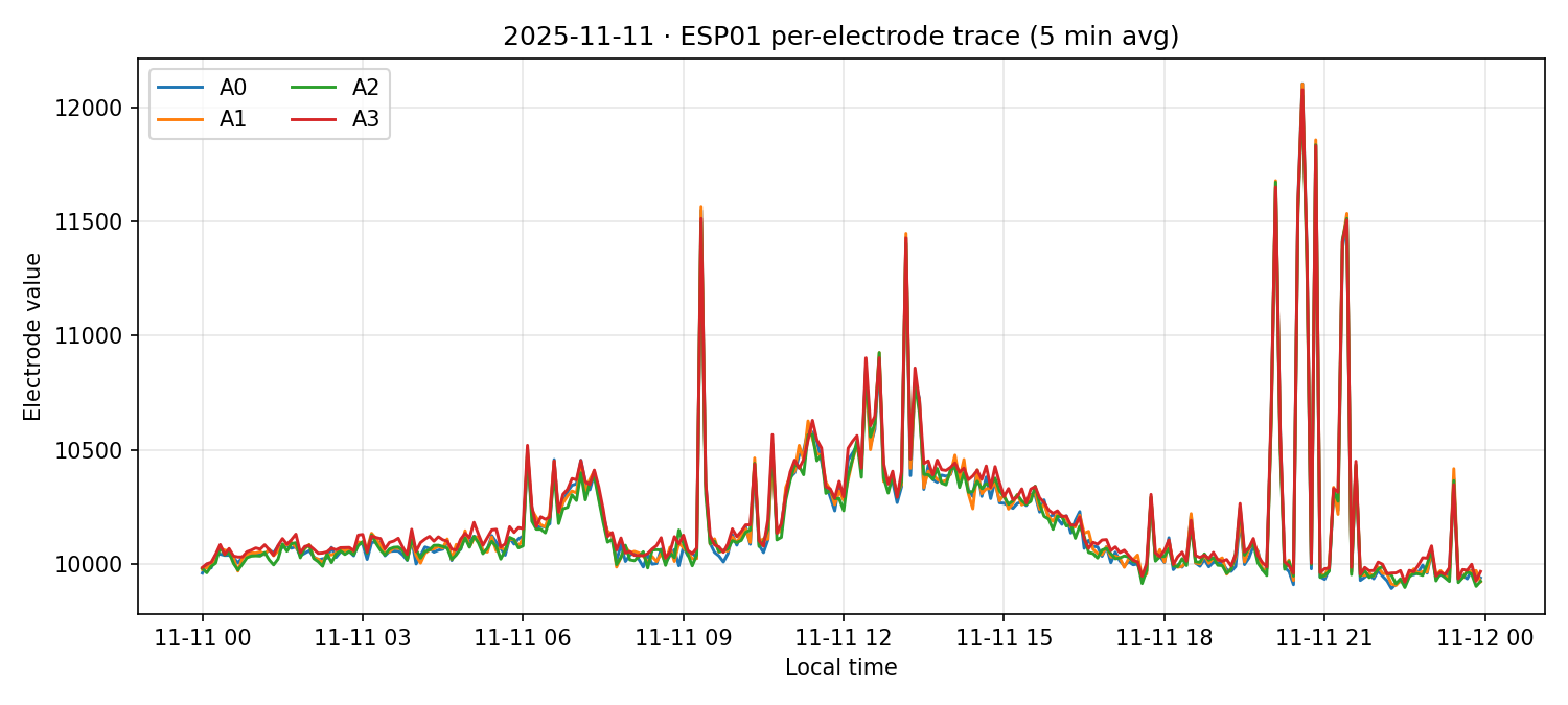
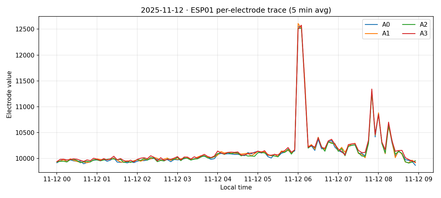
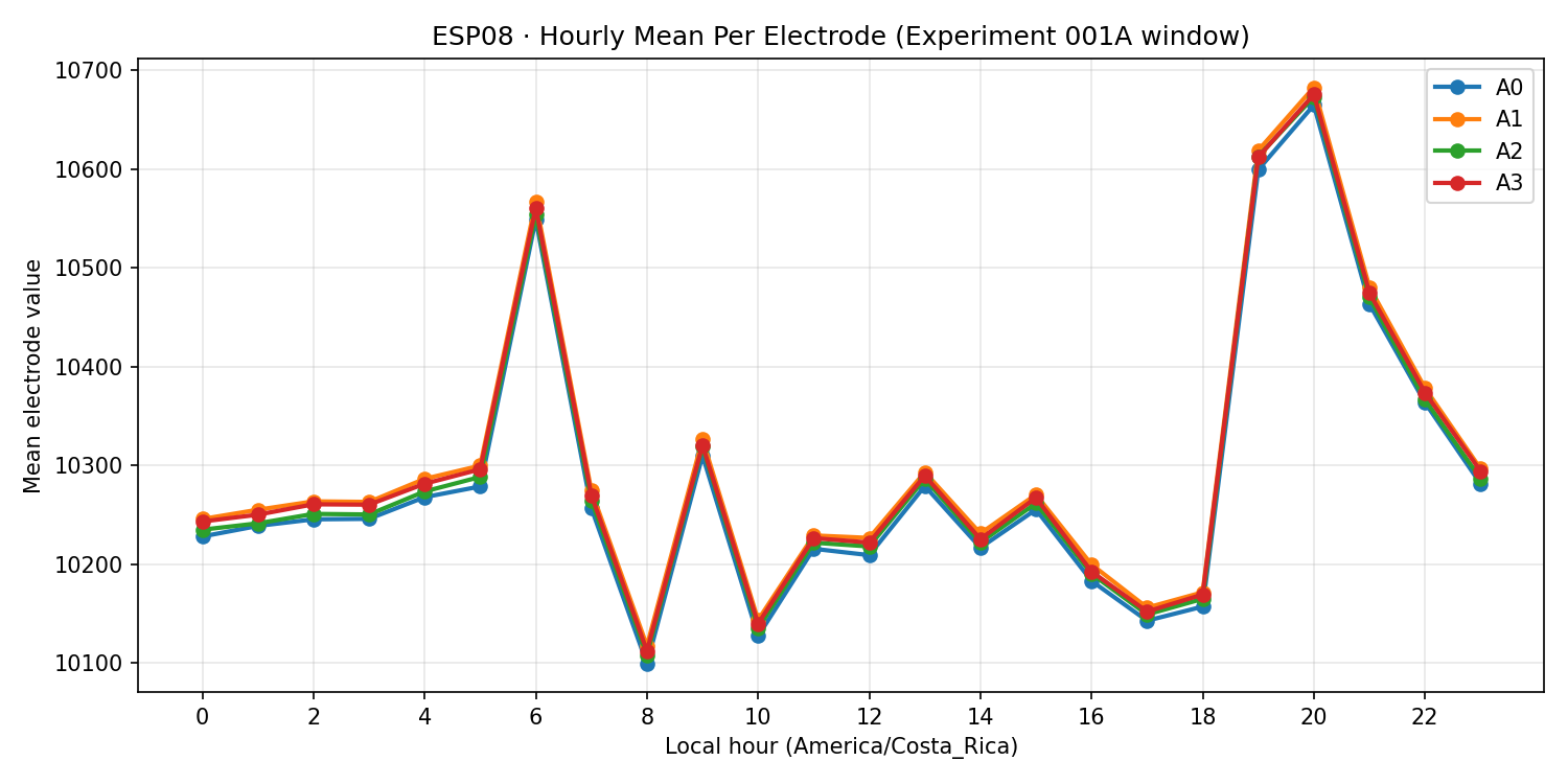
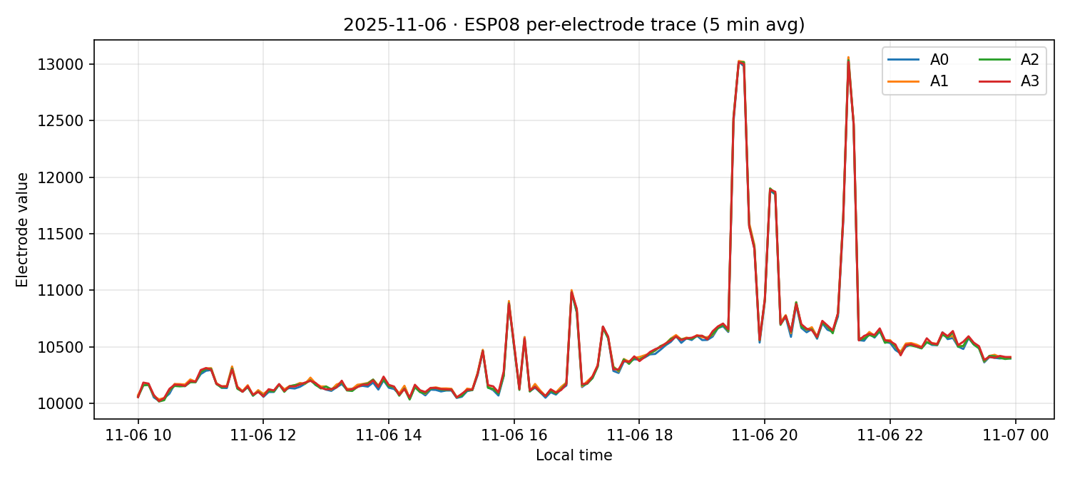
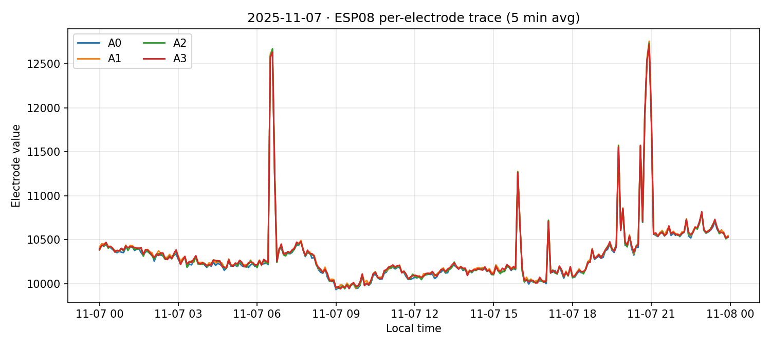
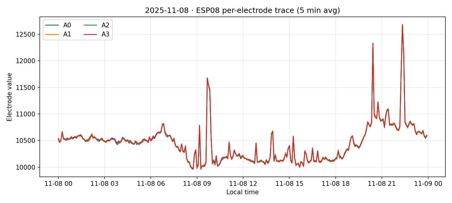
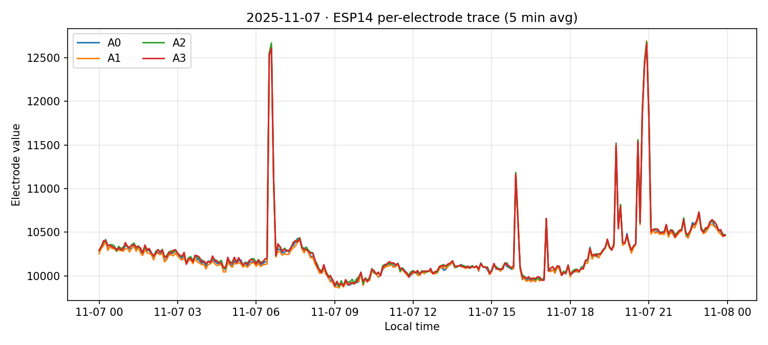
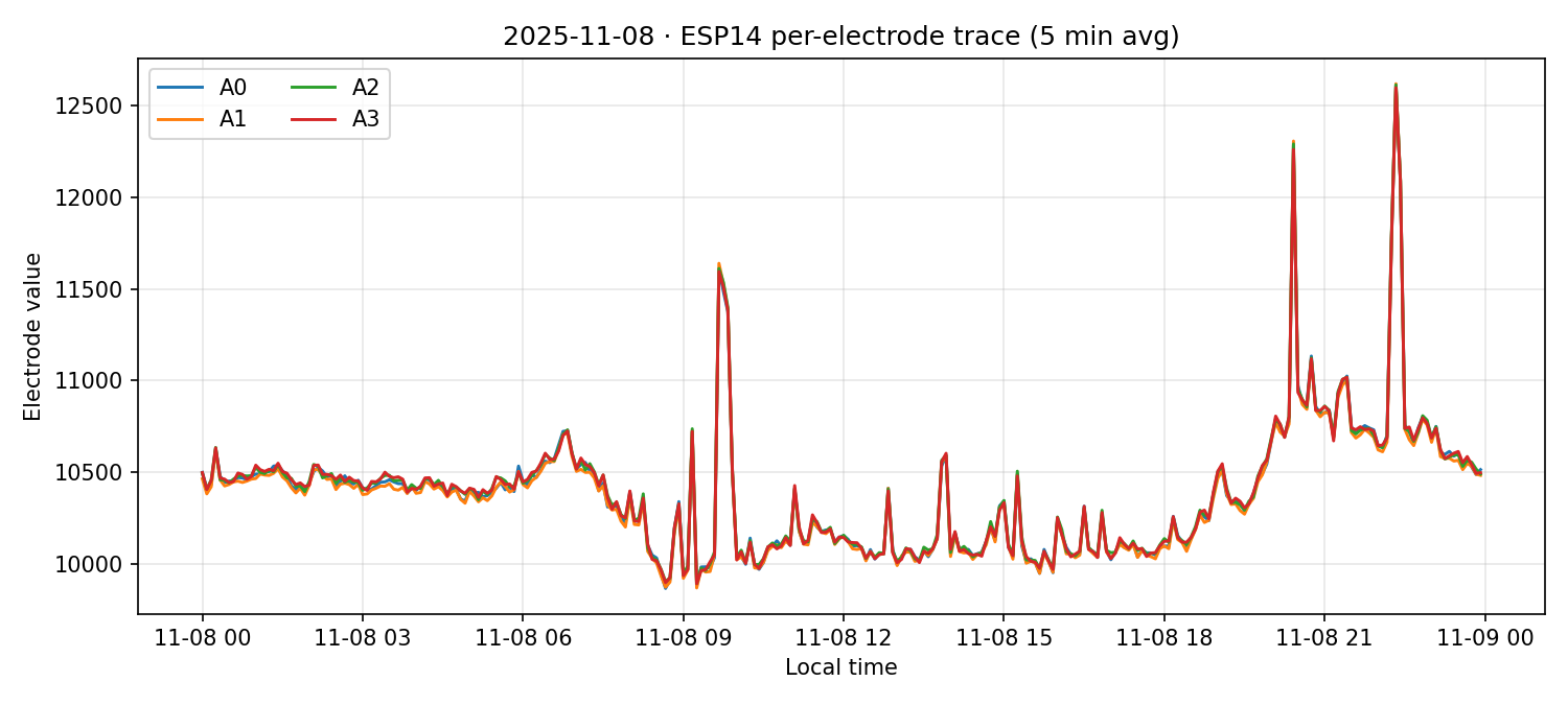
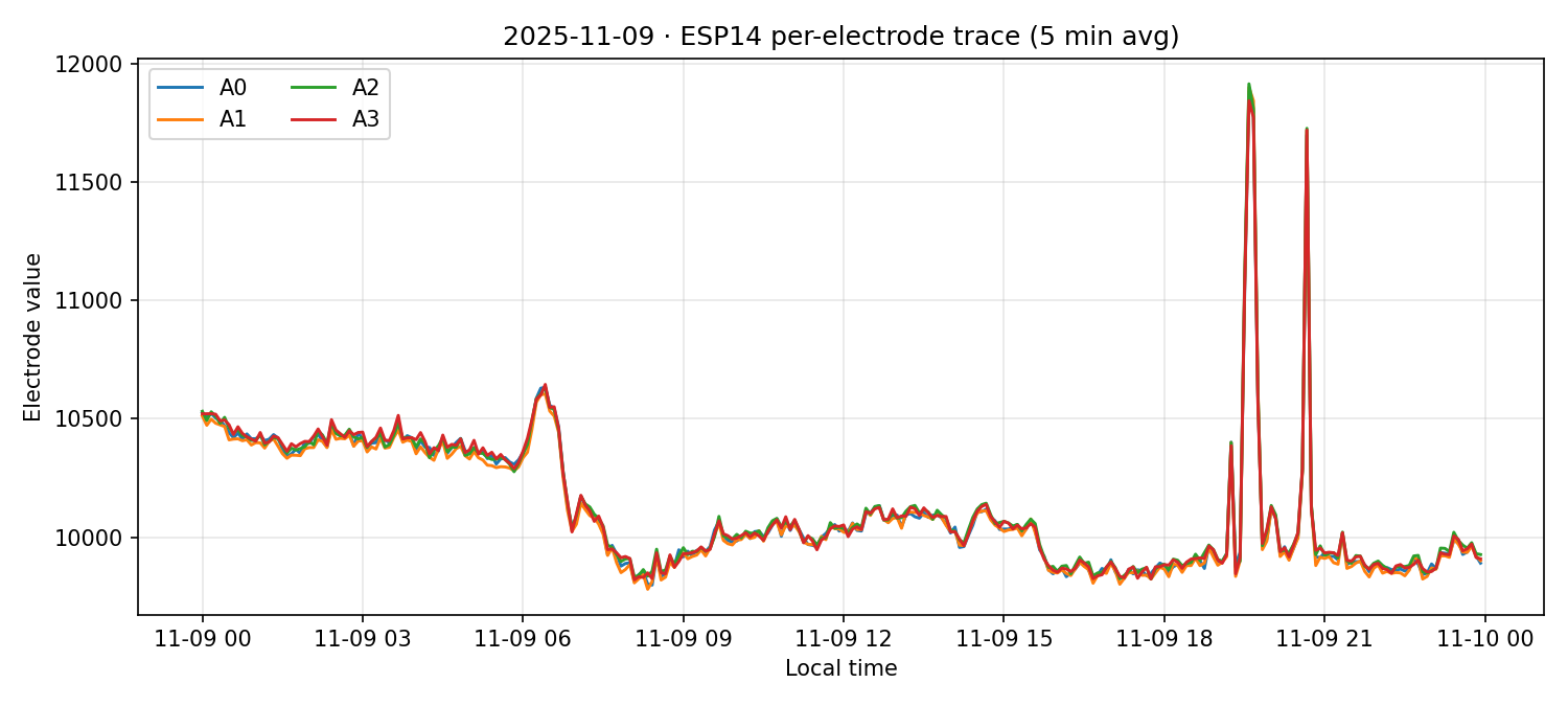
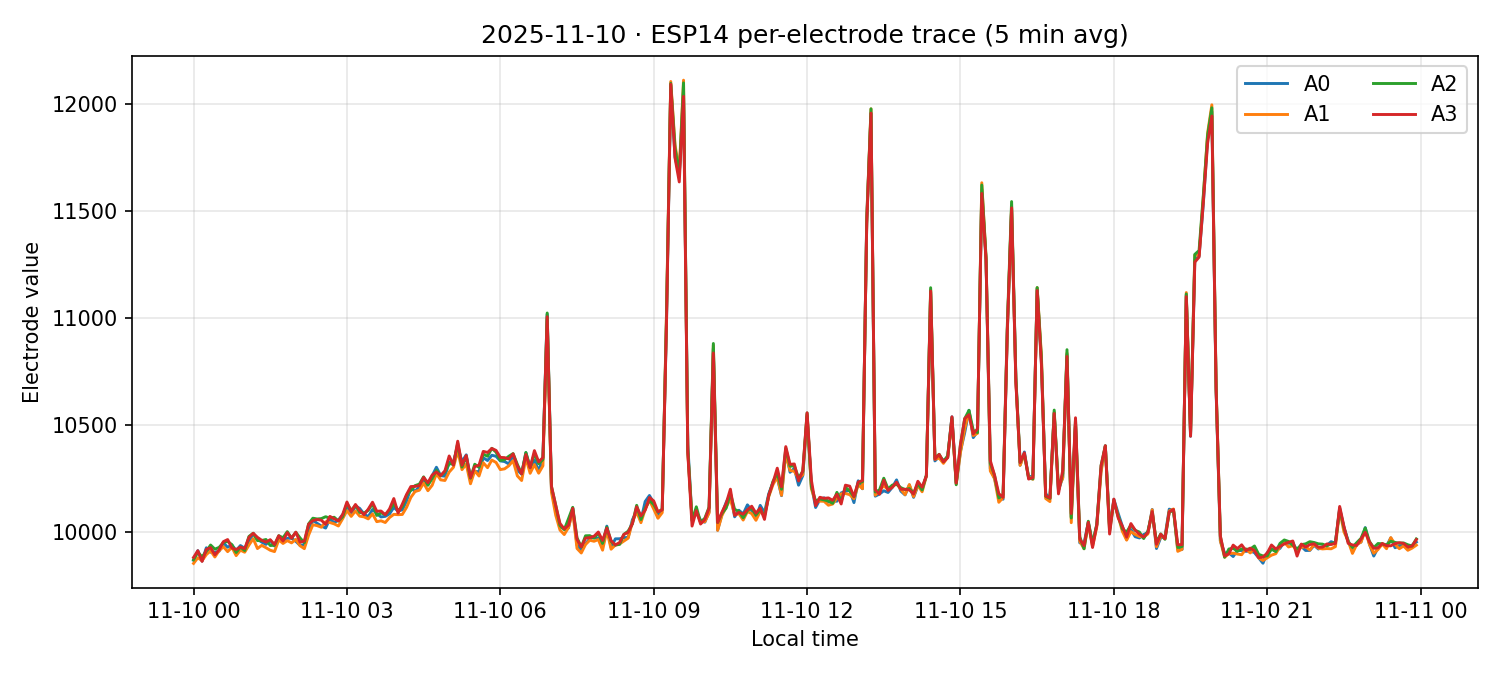
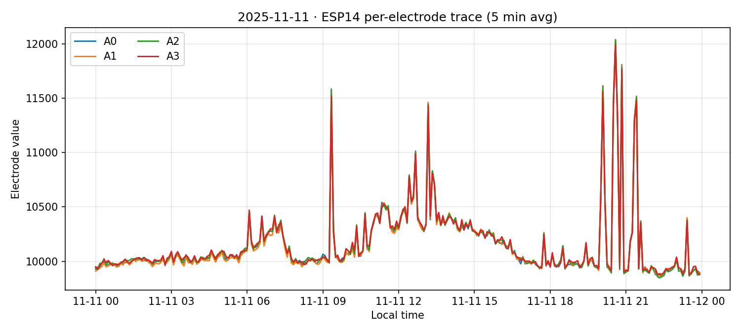
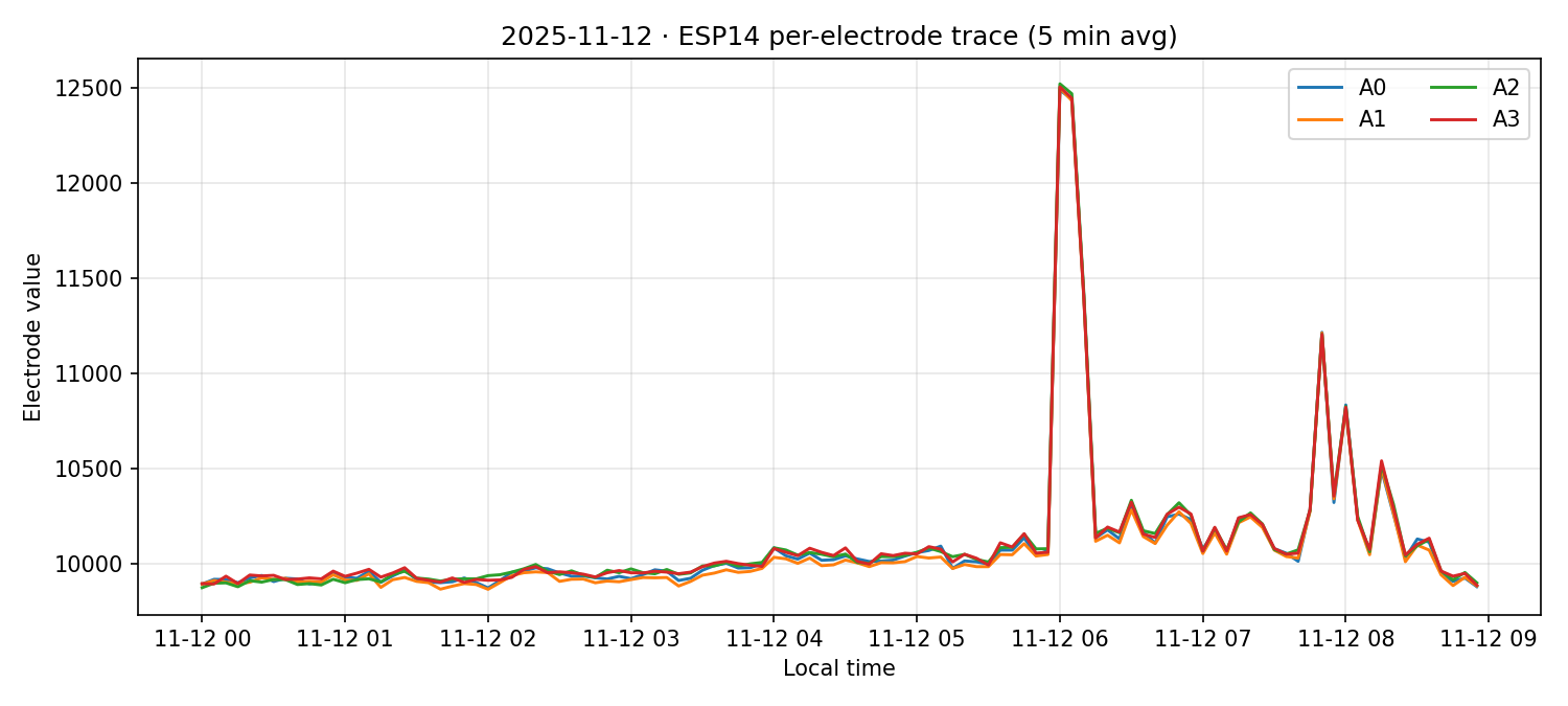
Approach. Using the 001A window (06 Nov 2025 16:01 UTC → 12 Nov 2025 15:00 UTC), we resampled each electrode (a0–a3) at 5 minutes, plotted per‑day traces, and quantified per‑timestamp spread as the standard deviation across the four electrodes, averaged over the window.
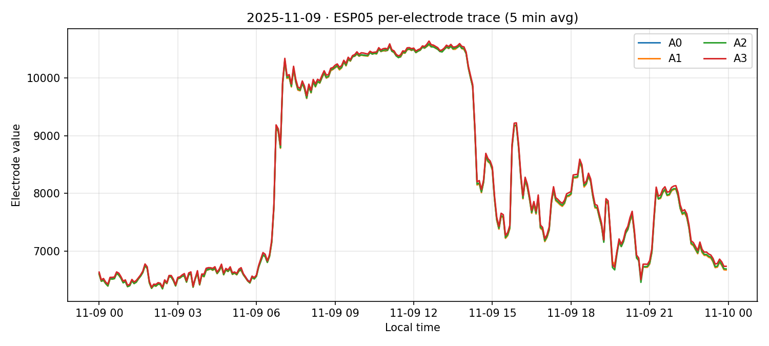
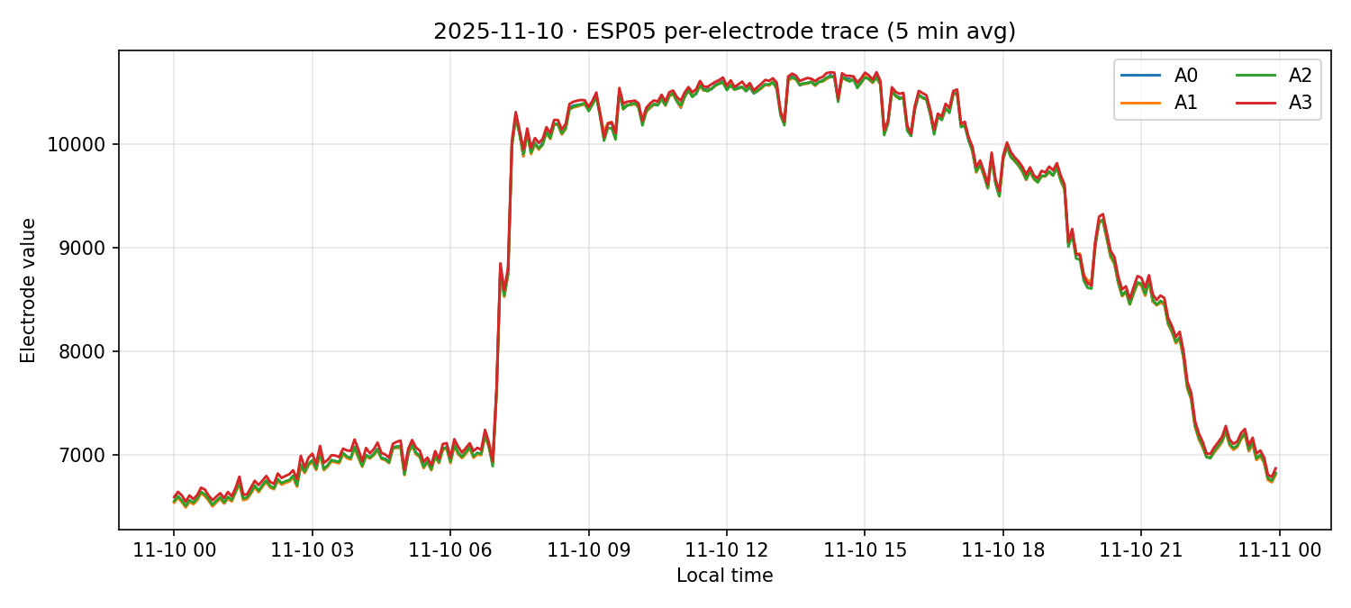
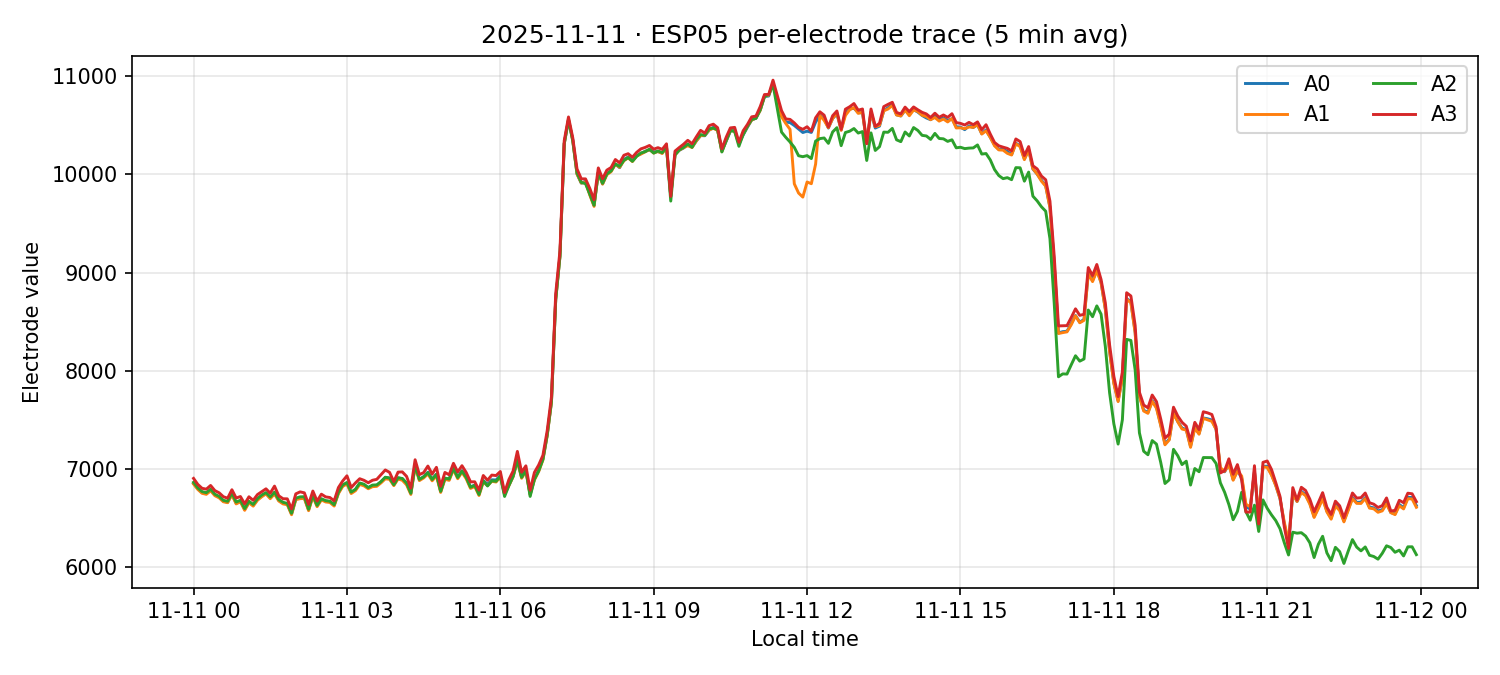
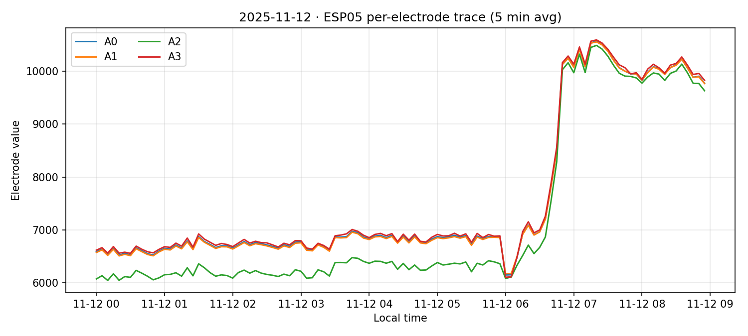
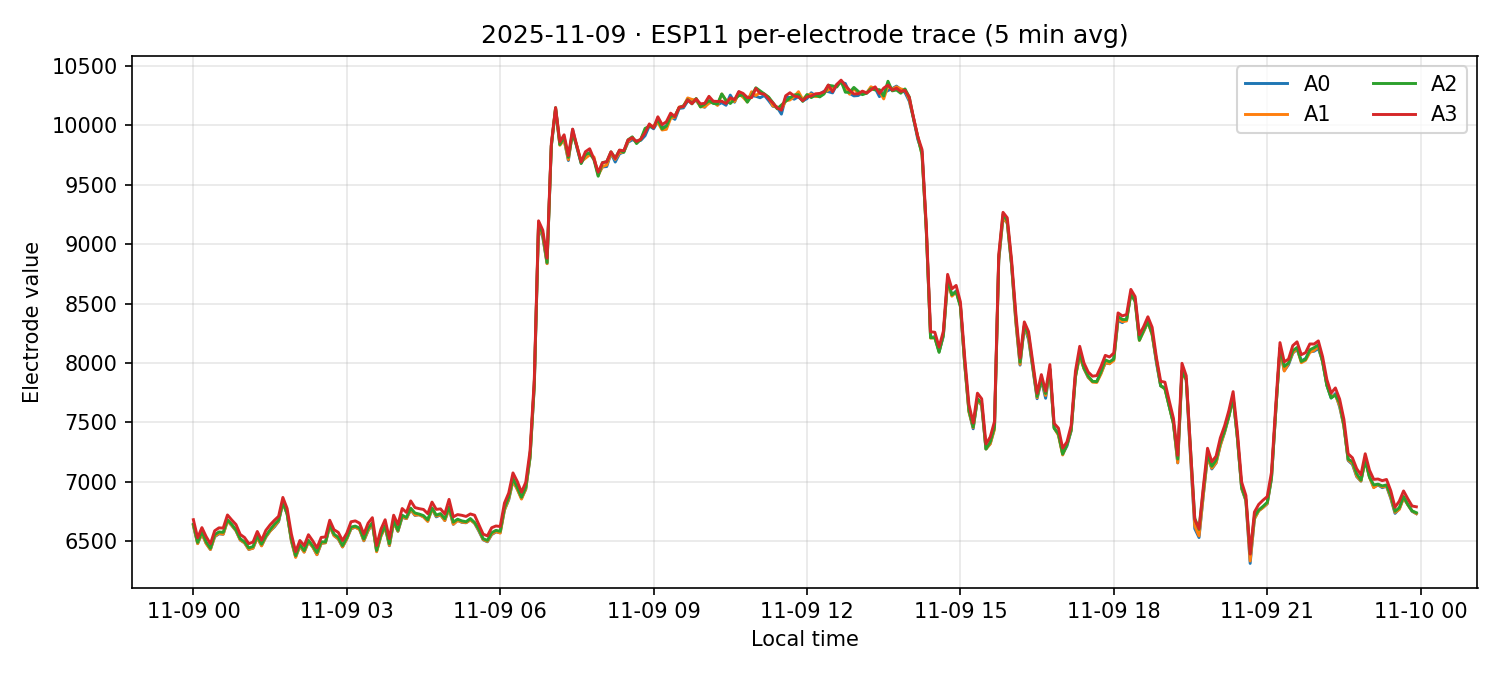
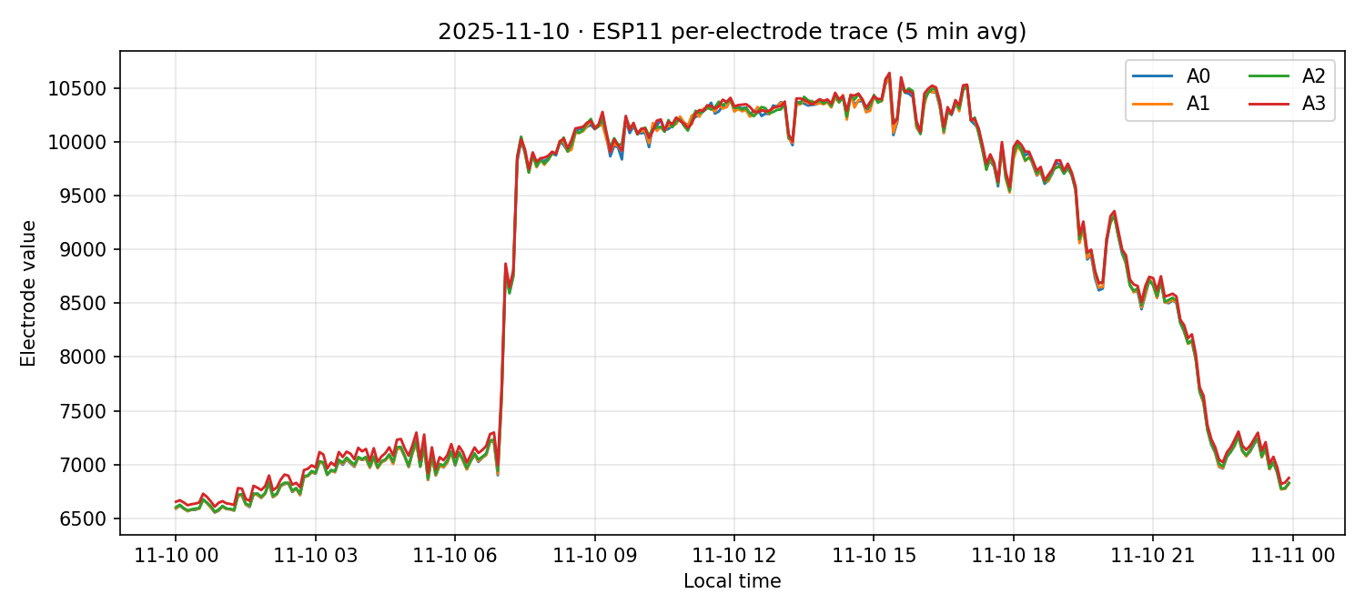
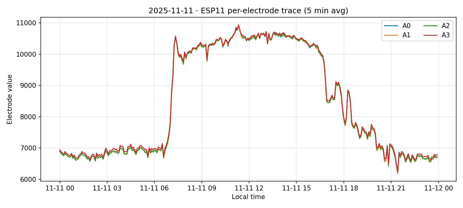
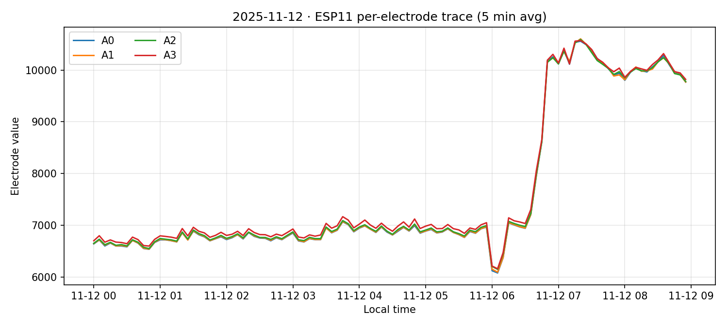
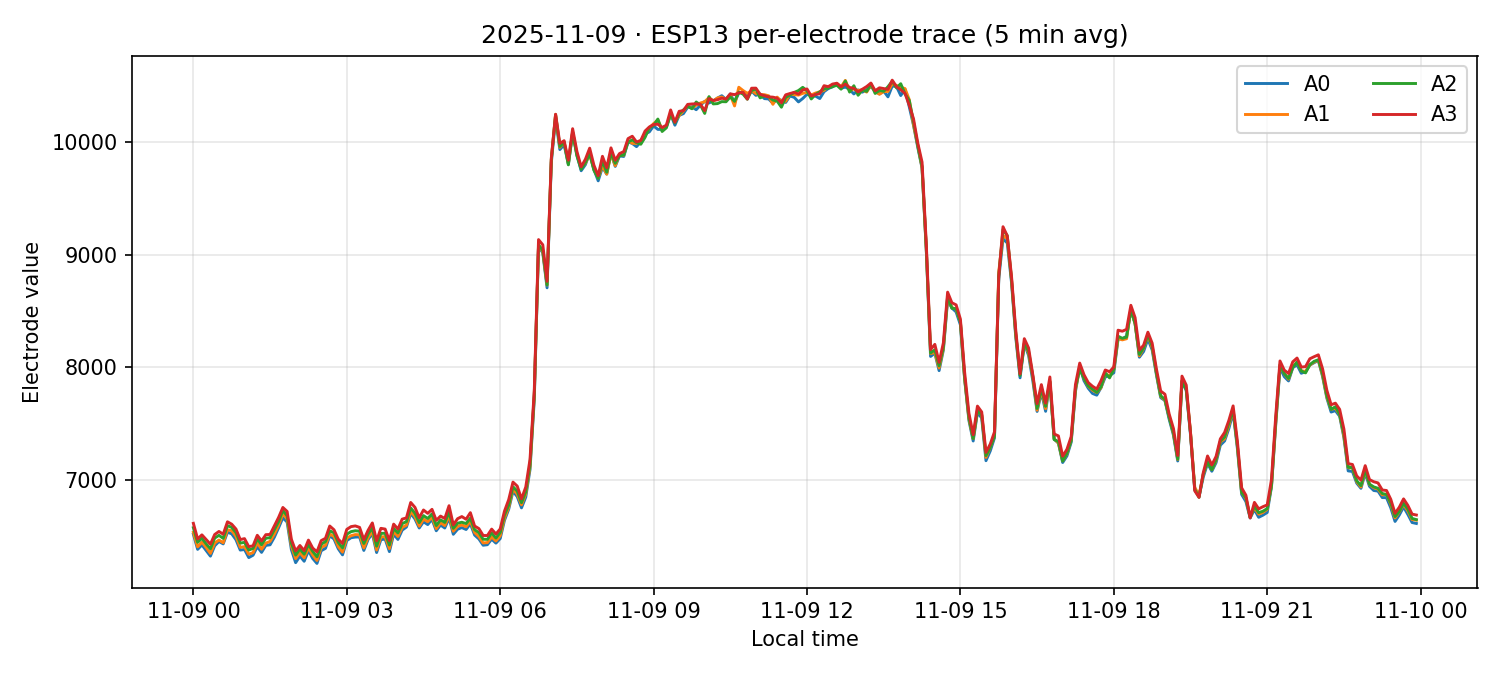
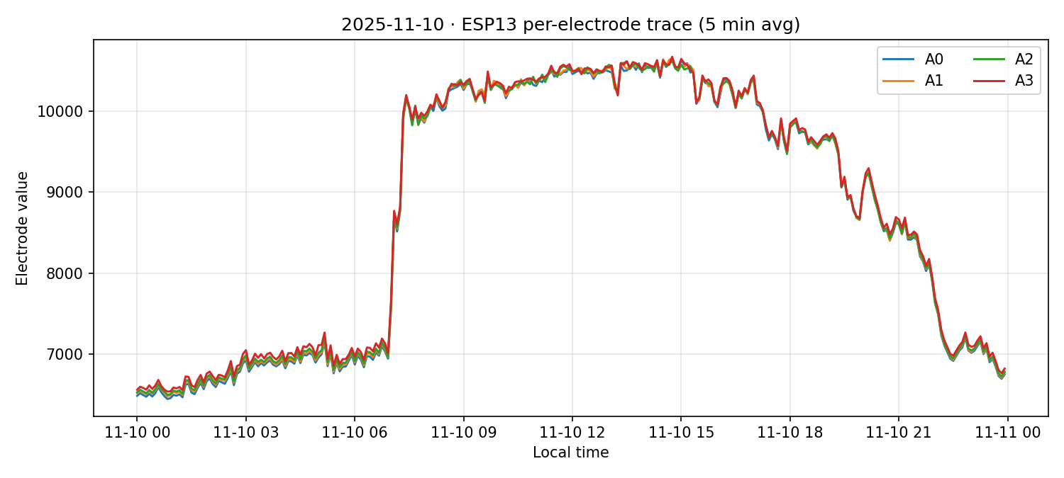
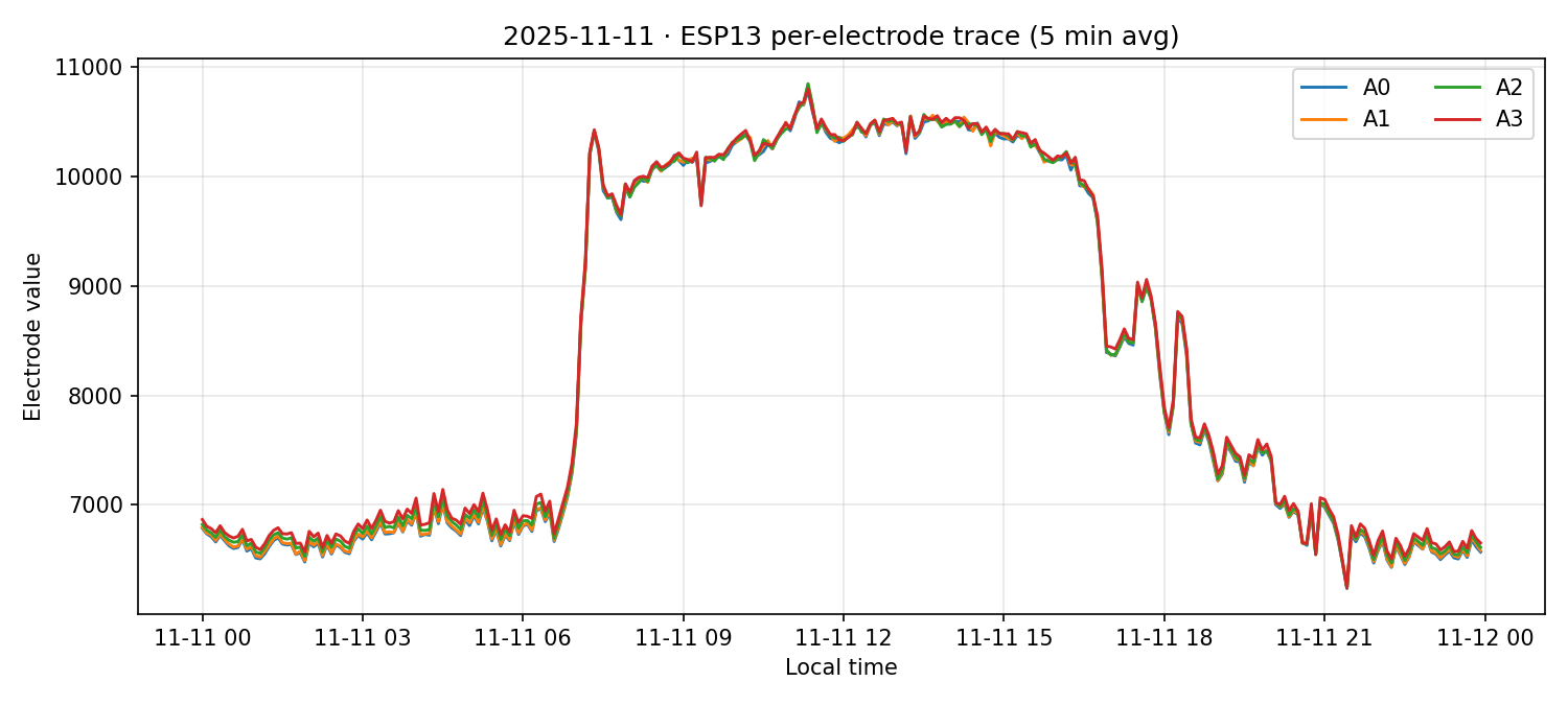
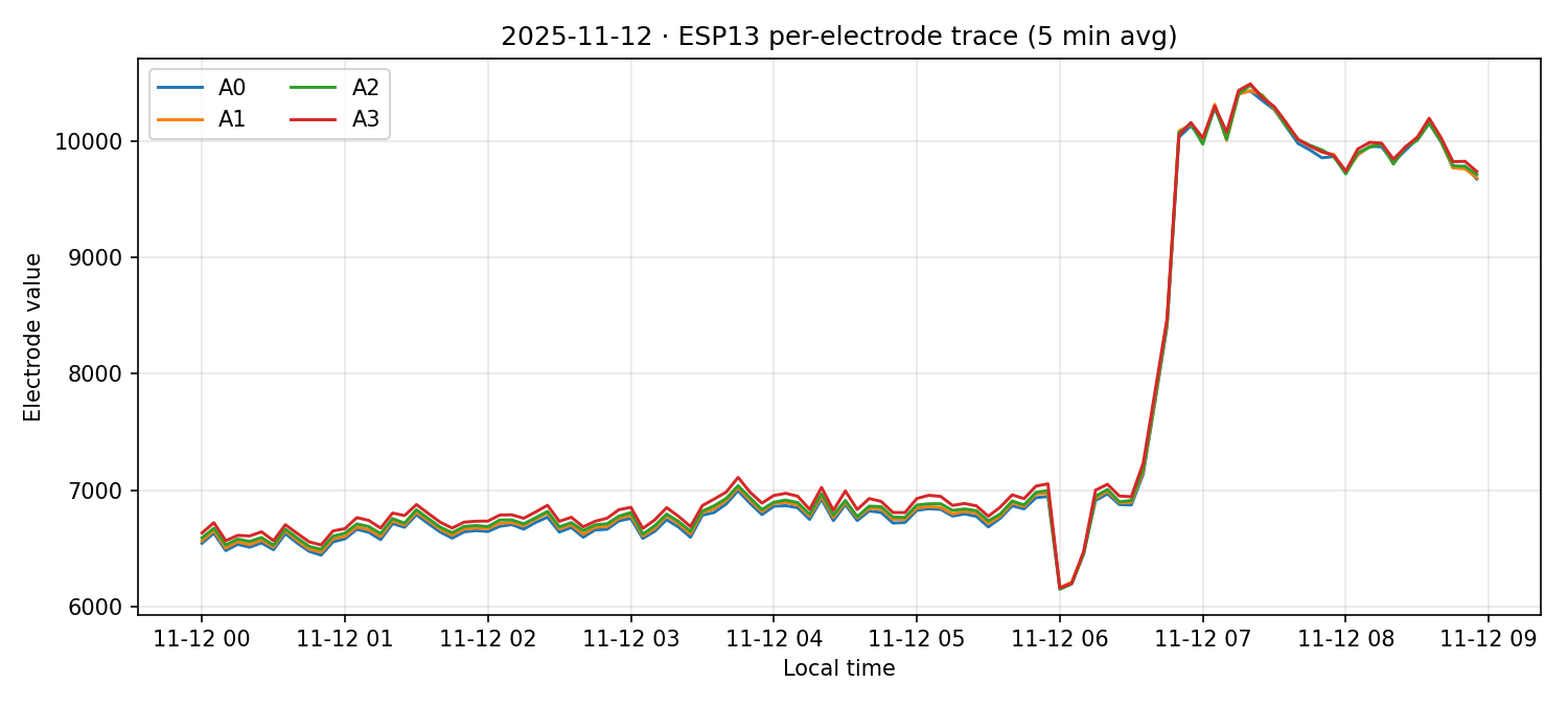
Results (Group 1 – ESP05/11/13). Mean spread across electrodes (counts): ESP05 ≈ 54.6 overall; ESP11 ≈ 84.3; ESP13 ≈ 88.1. ESP05 shows a notable episode: mean spread rises to ≈ 176.2 from 11 Nov 12:00 to 12 Nov 06:00, then moderates to ≈ 85.7 from 06:00–09:00 on 12 Nov. Throughout, the waveforms remain phase‑locked (AC‑coherent), even when the DC spread changes.
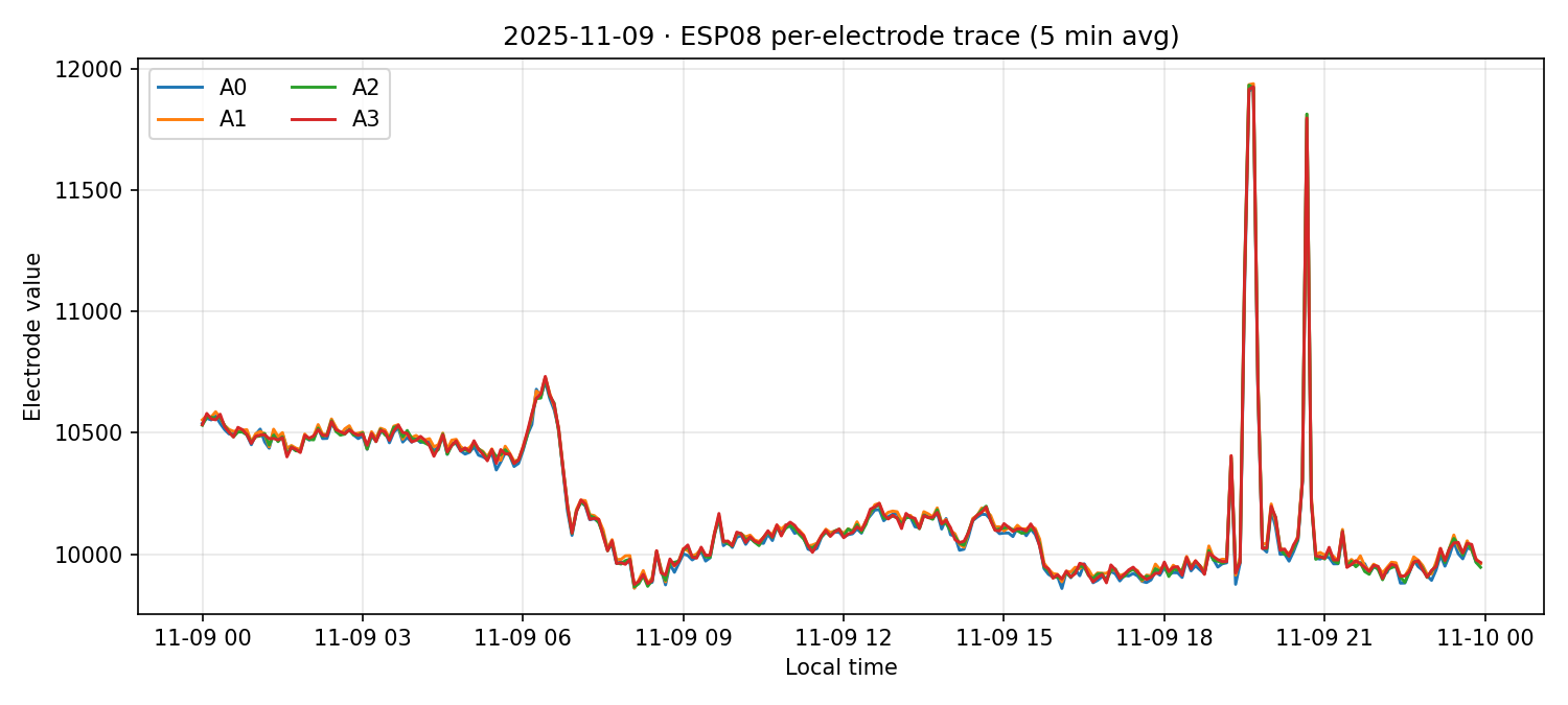
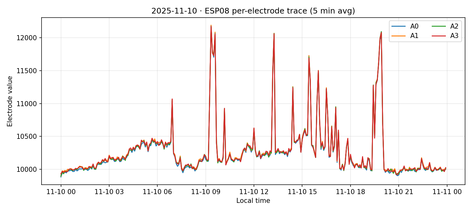
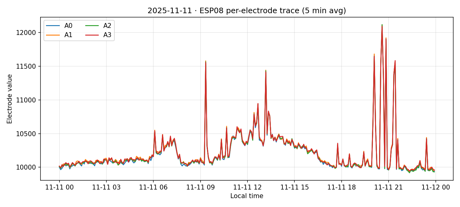
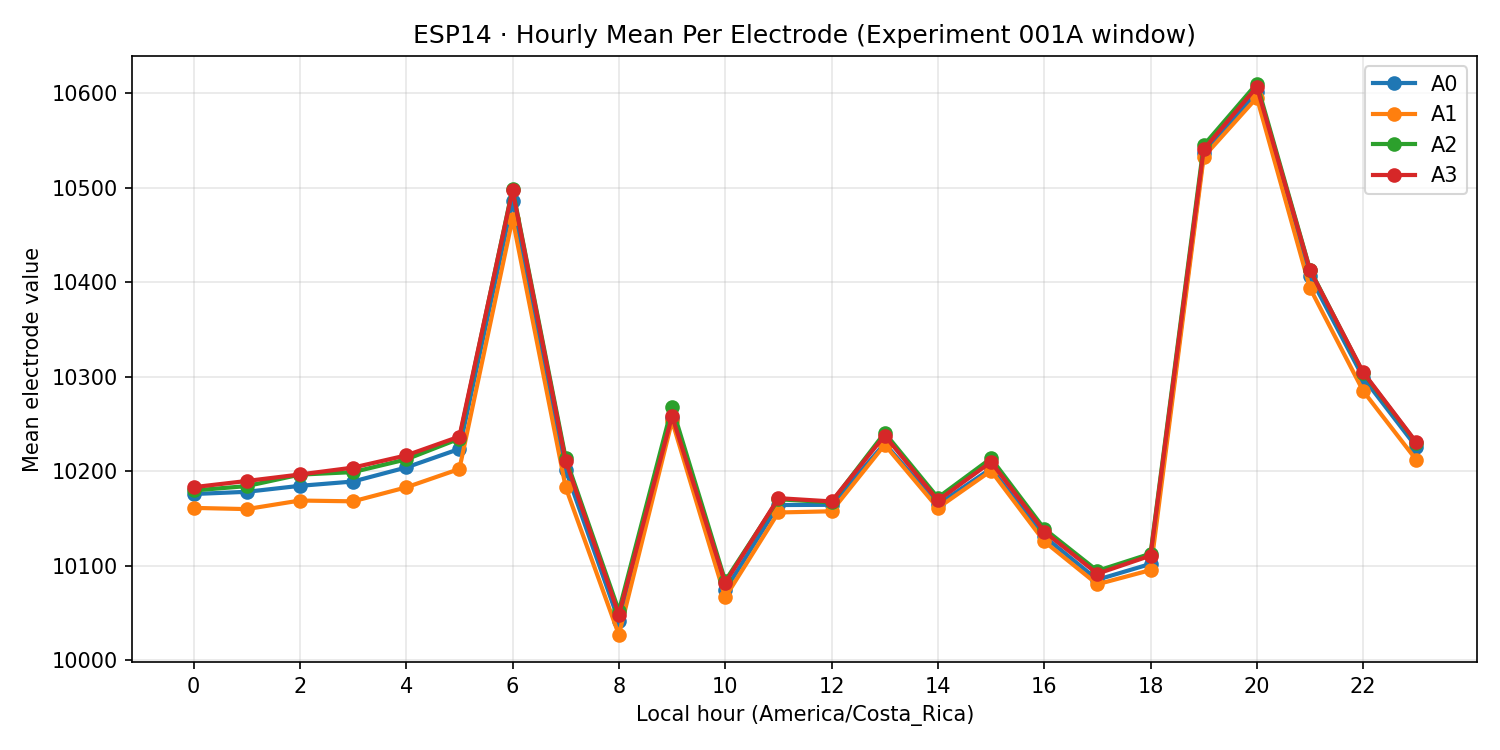
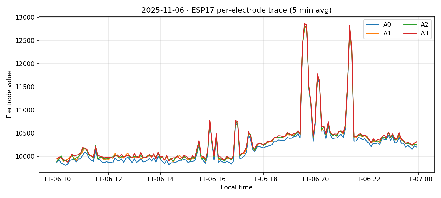
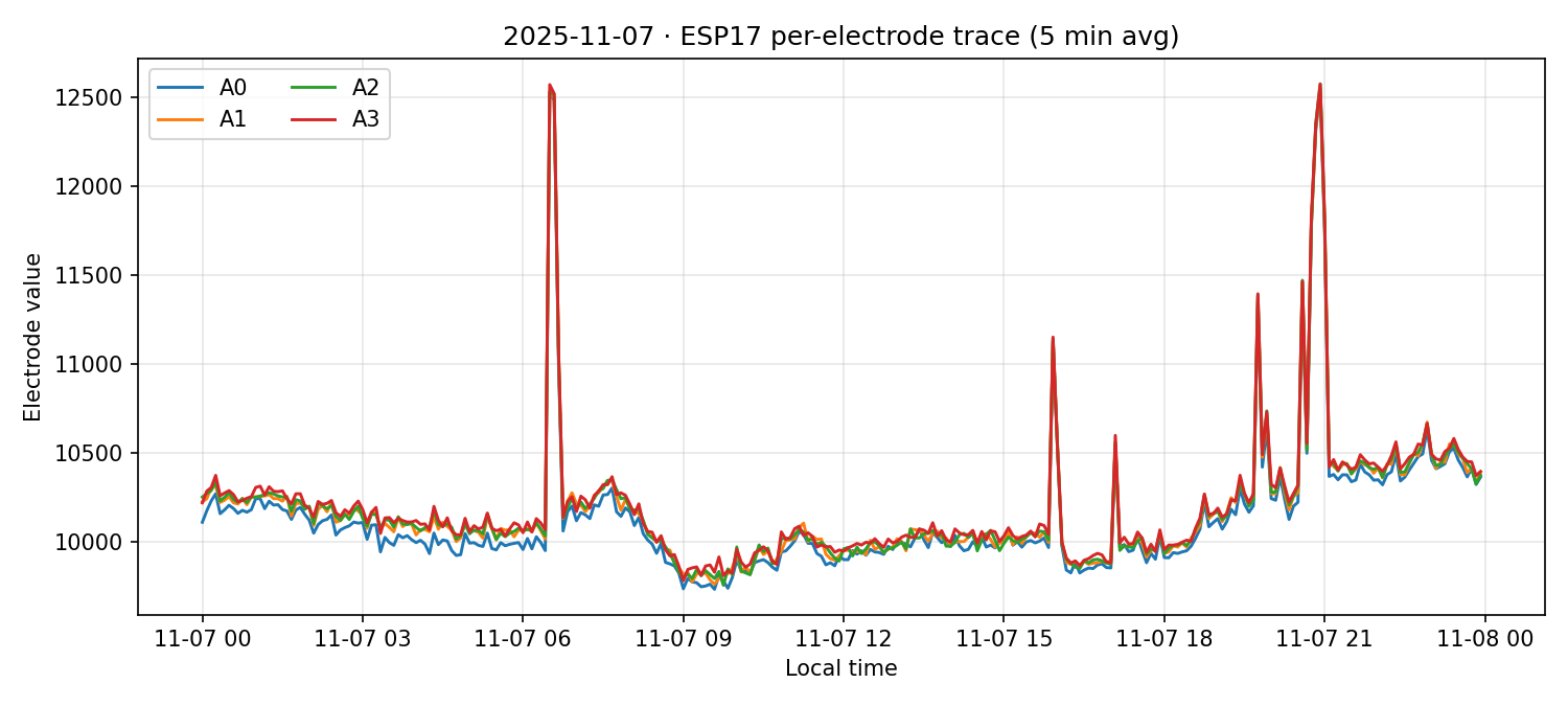
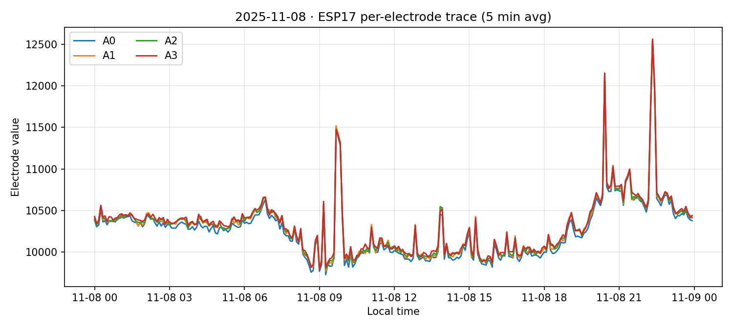
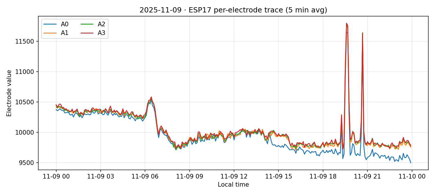
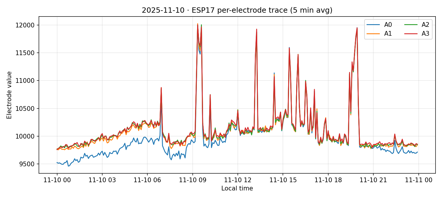
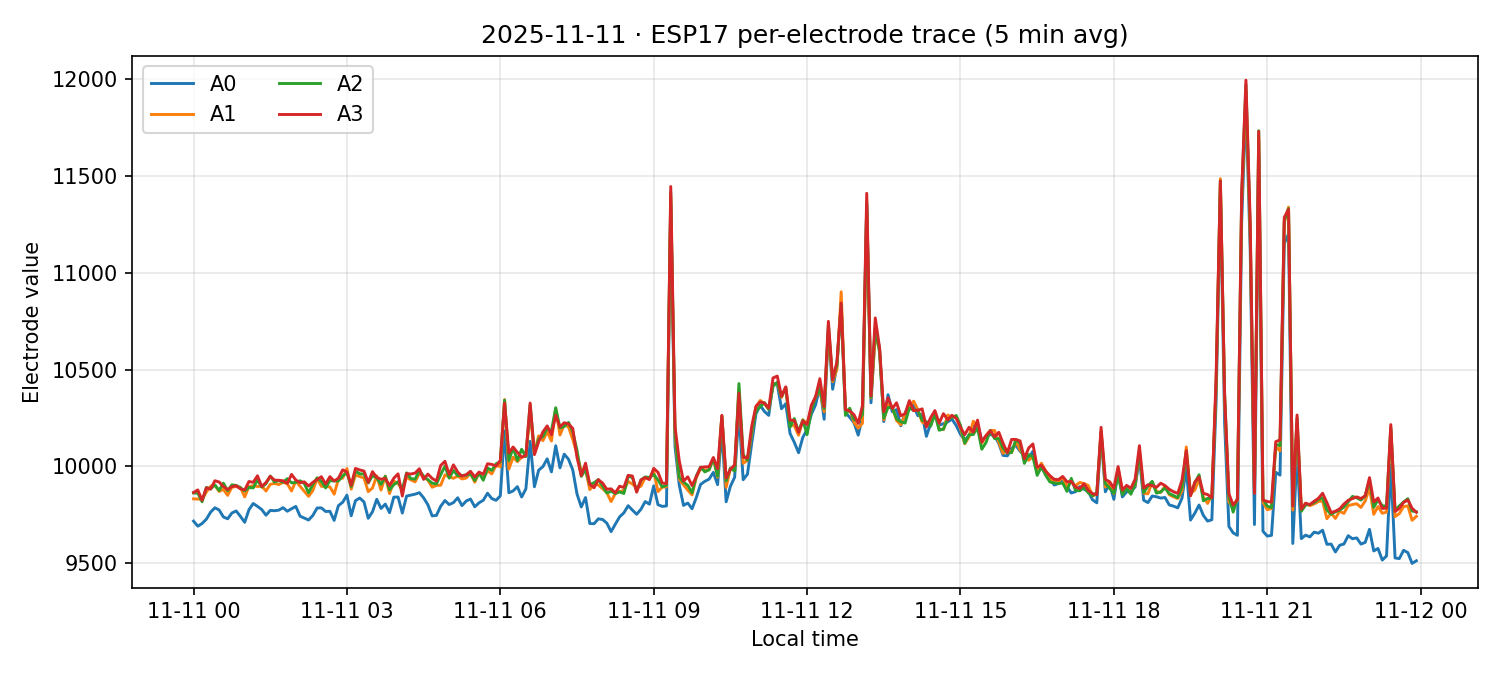
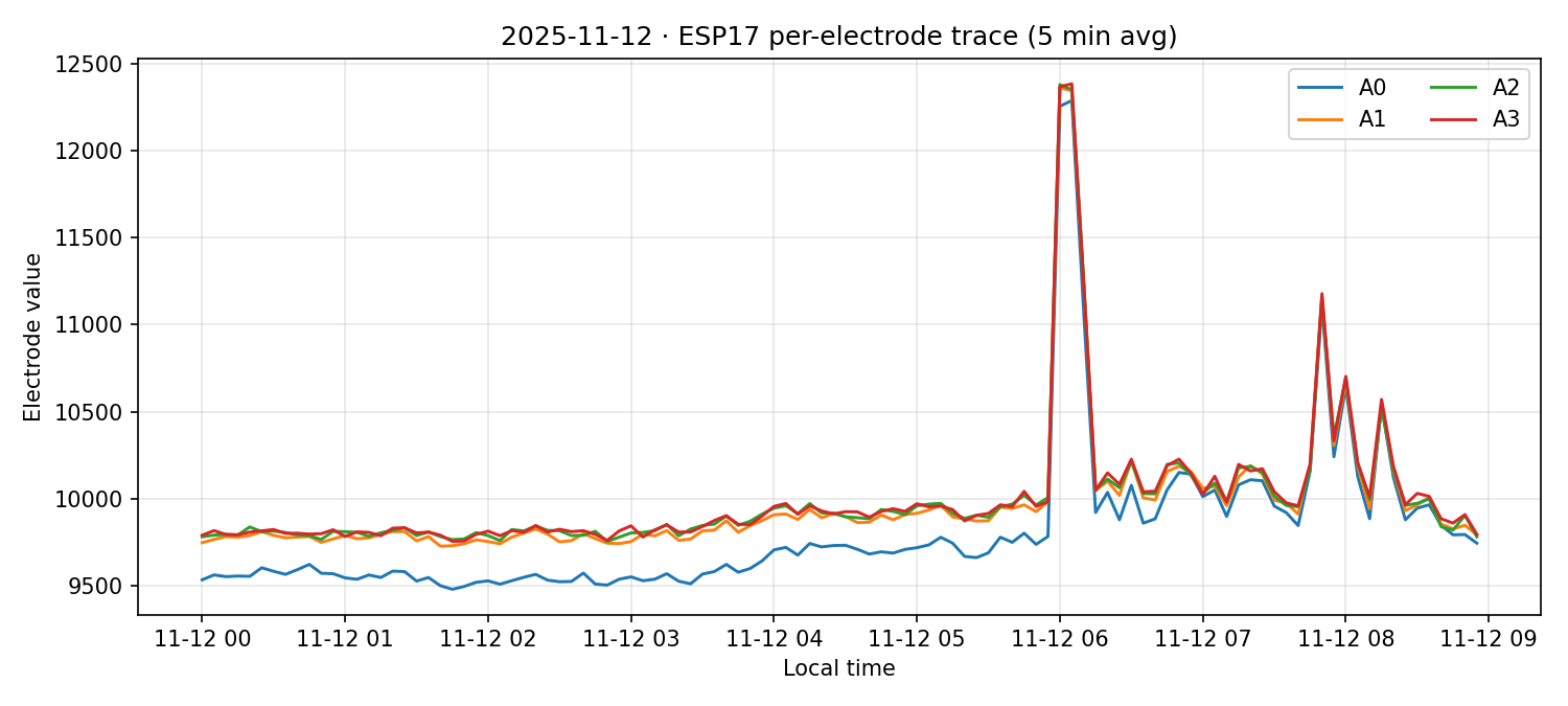
Results (Group 2 – ESP01/08/14/16/17). Similar to Group 1, devices exhibit periods of very low mean separation and periods of higher mean separation either across the full window or in specific segments. The phase remains matched, but the baseline separation drifts. Because we cannot yet ascribe biological meaning to these temporary differences, we do not extend per‑ESP deep‑dives here. Taken together, the data indicate members of a cluster tend to behave similarly overall; transient deviations are real but presently inconclusive.
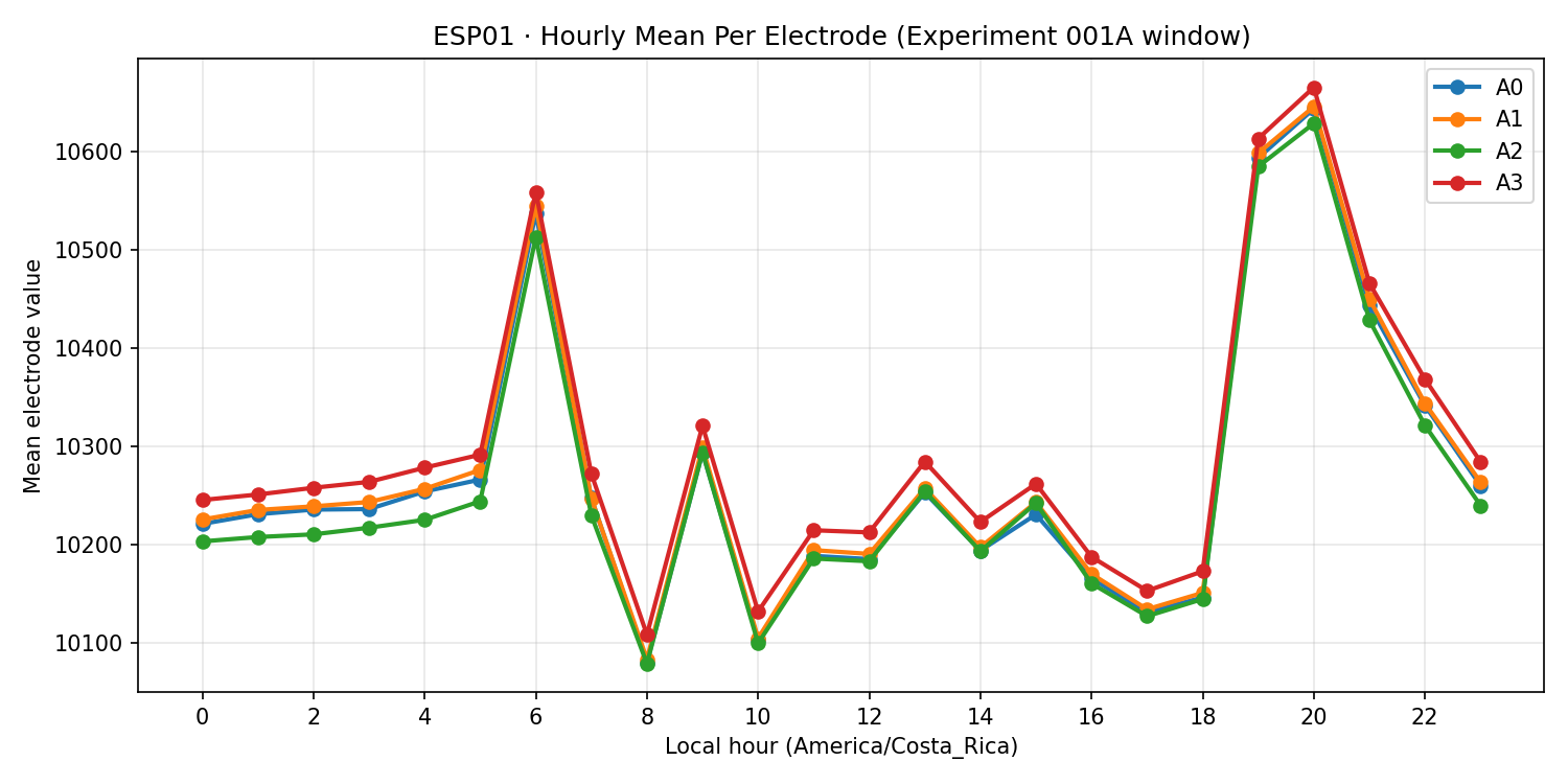
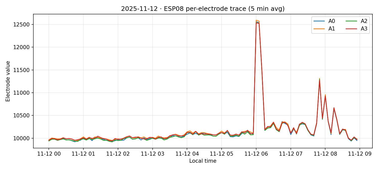
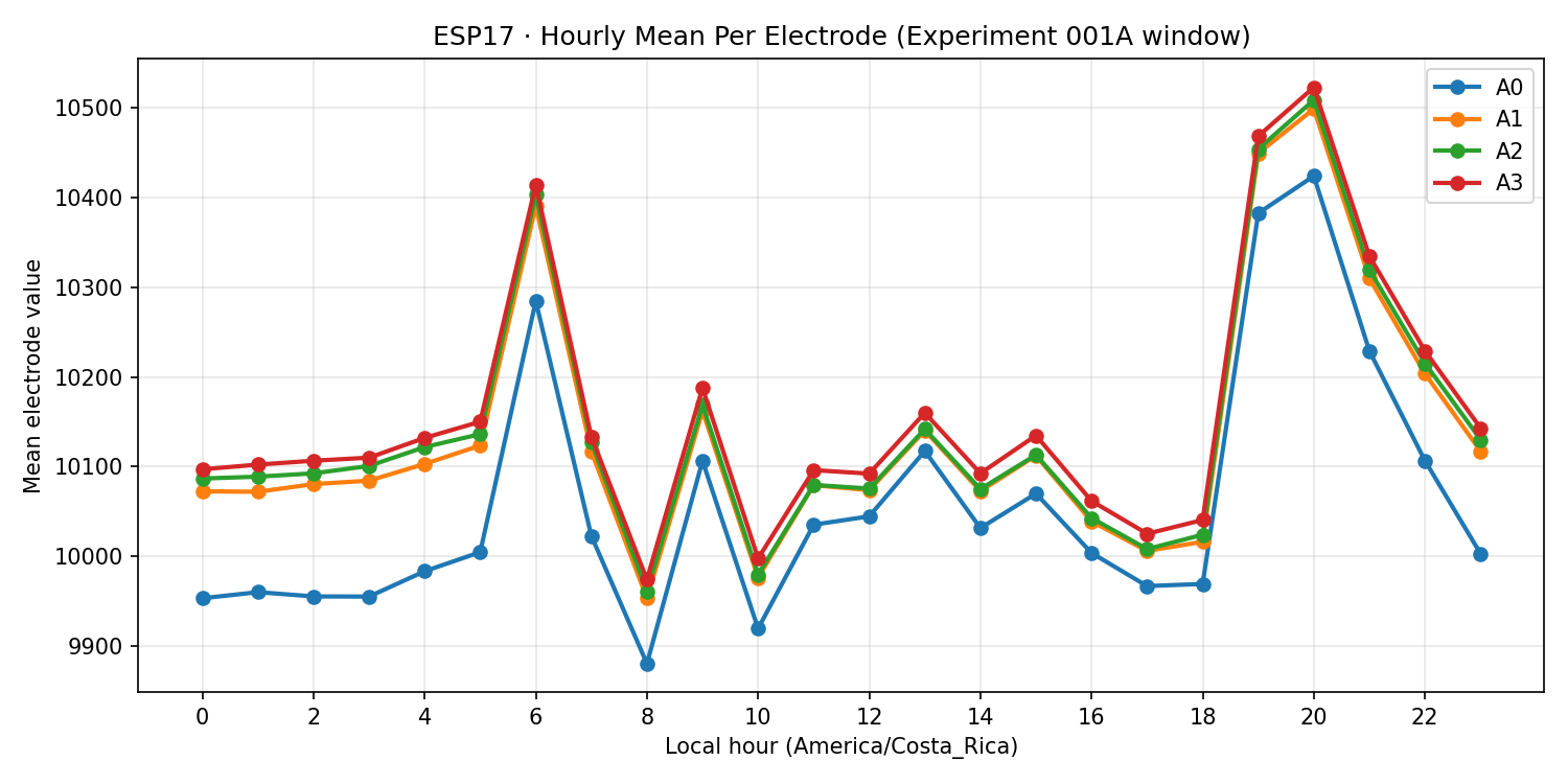
Group structure. The cluster split persists: Group 1 (ESP05/11/13) crests in late morning; Group 2 (ESP01/08/14/16/17) ramps toward evening, with ~500‑count daily dynamic range. Daily coverage stayed clean through 11 Nov, so these averages reflect full multi‑day coverage.
Conclusion. The per‑electrode data could potentially reveal a three‑level hierarchical model of fungal electrical activity: Level 1 (AC coherence) defines electrical domains—electrodes sharing the same AC rhythm likely belong to one coherent system; different AC patterns suggest separate domains. Level 2 (DC offset) marks local state within a domain—DC shifts with preserved AC coherence indicate a local operating point change (state to be characterized by FFT/PSD profiles). Level 3 (spikes) represents state‑dependent evoked responses—transient excursions on the DC baseline that vary with the underlying state. Per‑ESP electrodes are generally tightly clustered and phase‑coherent, supporting this framework.
Use the panels below to switch between ESPs and inspect each day individually.
Per-ESP panels
How to use. Choose an ESP from the menu, then scrub through the days with the slider. “Show all” restores the full week so you can compare days side-by-side.
ESP05
Group 1
06 Nov 2025
| Electrode | Samples |
|---|---|
| A0 | 21,370 |
| A1 | 21,370 |
| A2 | 21,370 |
| A3 | 21,370 |
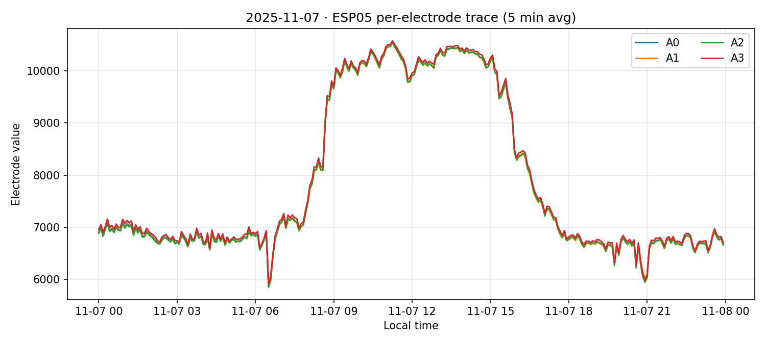
07 Nov 2025
| Electrode | Samples |
|---|---|
| A0 | 38,107 |
| A1 | 38,107 |
| A2 | 38,107 |
| A3 | 38,107 |
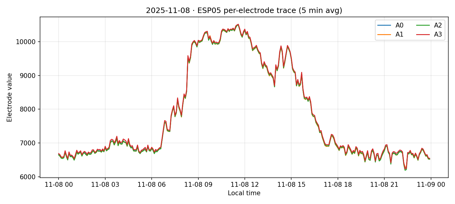
08 Nov 2025
| Electrode | Samples |
|---|---|
| A0 | 40,497 |
| A1 | 40,497 |
| A2 | 40,497 |
| A3 | 40,497 |
09 Nov 2025
| Electrode | Samples |
|---|---|
| A0 | 41,011 |
| A1 | 41,011 |
| A2 | 41,011 |
| A3 | 41,011 |
10 Nov 2025
| Electrode | Samples |
|---|---|
| A0 | 38,124 |
| A1 | 38,124 |
| A2 | 38,124 |
| A3 | 38,124 |
11 Nov 2025
| Electrode | Samples |
|---|---|
| A0 | 38,079 |
| A1 | 38,079 |
| A2 | 38,079 |
| A3 | 38,079 |
12 Nov 2025
| Electrode | Samples |
|---|---|
| A0 | 13,983 |
| A1 | 13,983 |
| A2 | 13,983 |
| A3 | 13,983 |

Saline comparison — per‑electrode (Oct 3–9, 2025)
Why compare. To check if per‑electrode spreads seen in fungus also appear in hardware‑only saline, we plotted a0–a3 per day for the saline bath (3–9 Oct). If electrodes stay phase‑matched but baselines separate with heat/evaporation, that indicates interface/environment rather than biology.
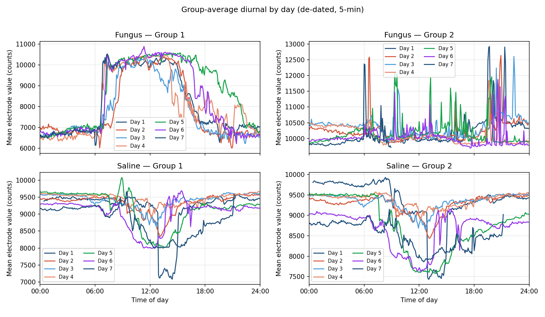
Group‑average diurnal overlays. We now include consolidated group lines to make the patterns clear at a glance:
- Fungus vs Saline (4‑line overlay). Two fungus groups (solid) and two saline groups (dashed) over the same time‑of‑day axis.
- By‑day (de‑dated) panels. Each day is relabeled Day 1/2/3 and overlaid so shapes can be compared independent of calendar dates.
Saline per‑electrode — averaged over Oct 3–9
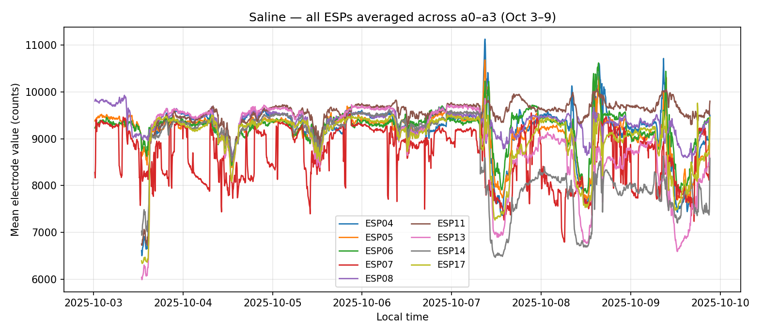
All saline ESPs — averaged across a0–a3 (Oct 3–9)
This overlay shows each ESP as a single trace (mean of a0–a3) over the full saline period, so you can compare devices directly.
Scripts used. Extraction: analysis/fungal_state_mapping/scripts/extract_saline_per_electrode_range.py. Plotting & metrics: analysis/fungal_state_mapping/scripts/generate_saline_per_electrode_plots.py. Same 5‑minute resampling approach as 001B.
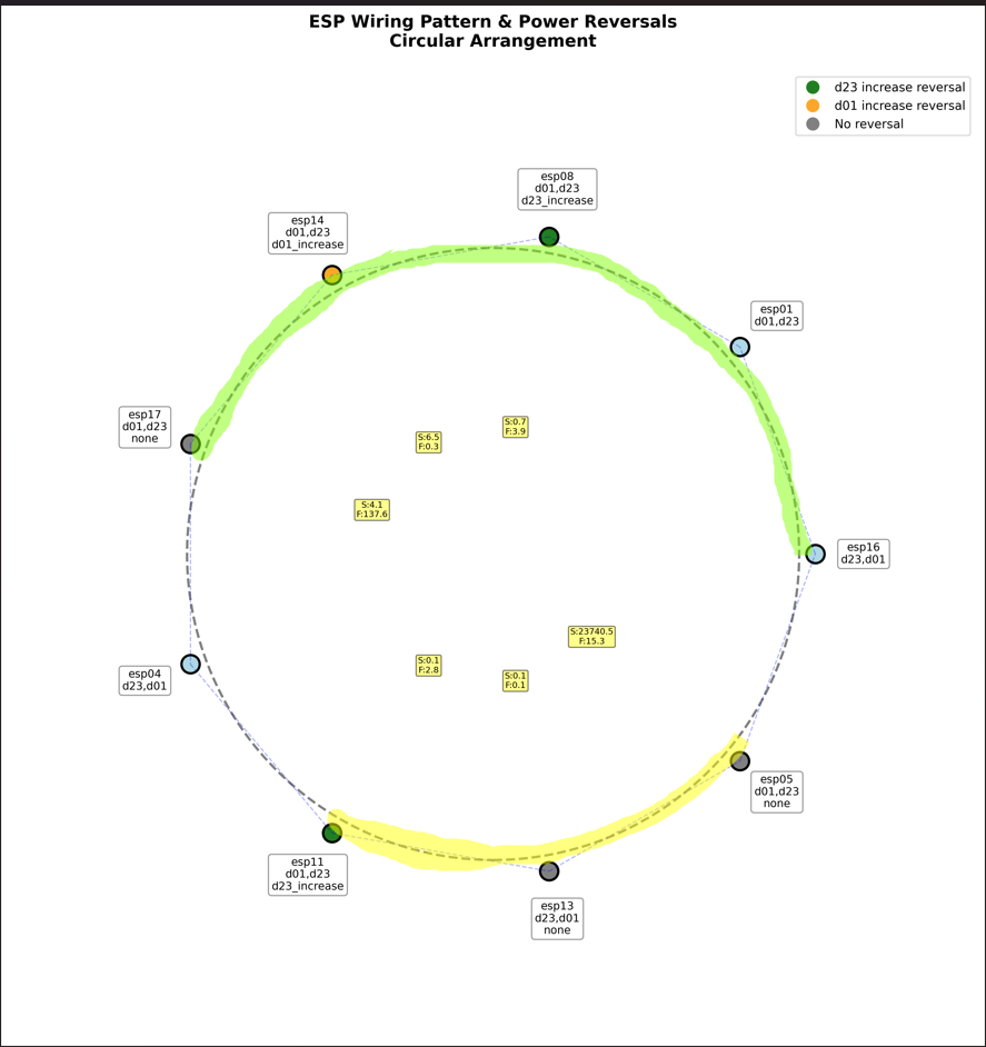
Wiring reference
Fungus vs Saline Spread Comparison
Quantitative comparison of electrode spread patterns. A detailed statistical analysis comparing electrode spread (standard deviation of a0–a3) between the living fungus baseline (Nov 6–12) and saline control periods (Oct 3–9, split into early Oct 3–6 and late Oct 7–9). This analysis addresses whether high-spread episodes in living fungus are statistically and visually similar to saline evaporation/heat artifacts.
Analysis & Findings (Analyzed by AI)
Extended analysis: Multi-run per-electrode profiles. To test whether electrodes track together in a single connected substrate (as one pool of saline resembles one block of fungus), we extended the per-electrode analysis to Experiment 003's three runs: cups configuration, bottle outdoor, and bottle AC room. Results confirm that electrodes track together in the single-pool configurations, supporting the hypothesis that a connected substrate (whether saline or fungal) produces coherent electrode behavior. View extended multi-run analysis →
Within-ESP coherence. Across all panels, the four electrodes on a single ESP travel within ±40 raw counts of one another during active periods. ESP05 and ESP11 show the tightest synchrony (a0–a3 curves nearly overlapping), implying that the lower-mounted probes are sampling a homogeneous micro-zone. ESP01/08/14/16/17 exhibit slightly larger spreads late in the evening (a2 tends to run ~60 counts lower than a0/a1), but the phase remains matched throughout the extension window.
Temporal drift. Group 1 devices peak between 10:30–11:30 local time every day; the slider reveals less than 5 % amplitude drift through 11 Nov, followed by the expected attenuation on 12 Nov when acquisition was curtailed. Group 2 devices rise steadily after 16:00, reaching maxima between 19:30–21:00. The per-day plots highlight a reproducible shoulder near 05:00–06:00 where the elevated electrodes reset before the next build-up.
Data quality. The sample-count tables under each plot confirm full channel availability for every active day (all four electrodes report identical counts). Coverage drops uniformly on 12 Nov—the final operational day—so subsequent analyses should either trim that date or treat it separately.
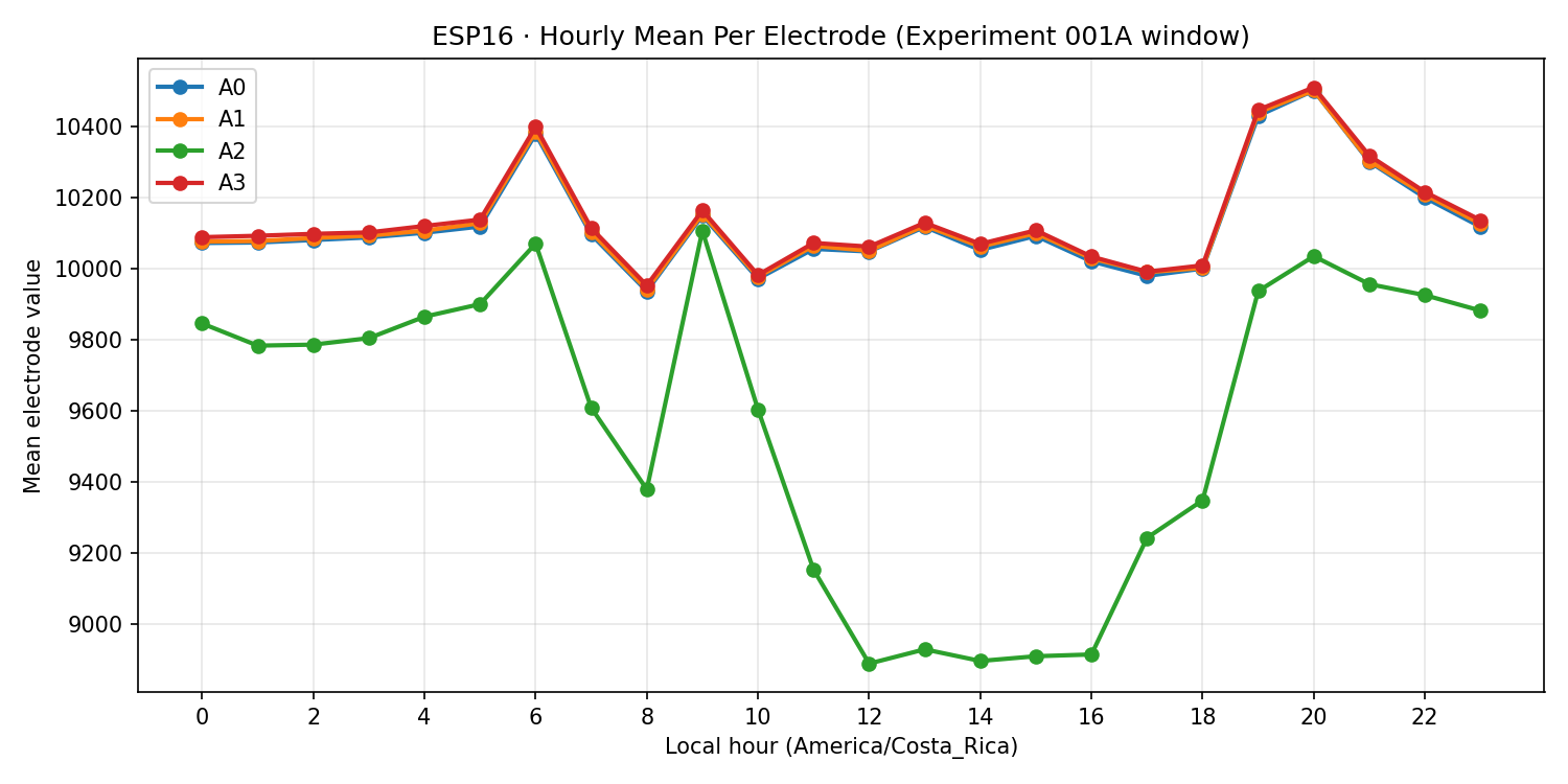
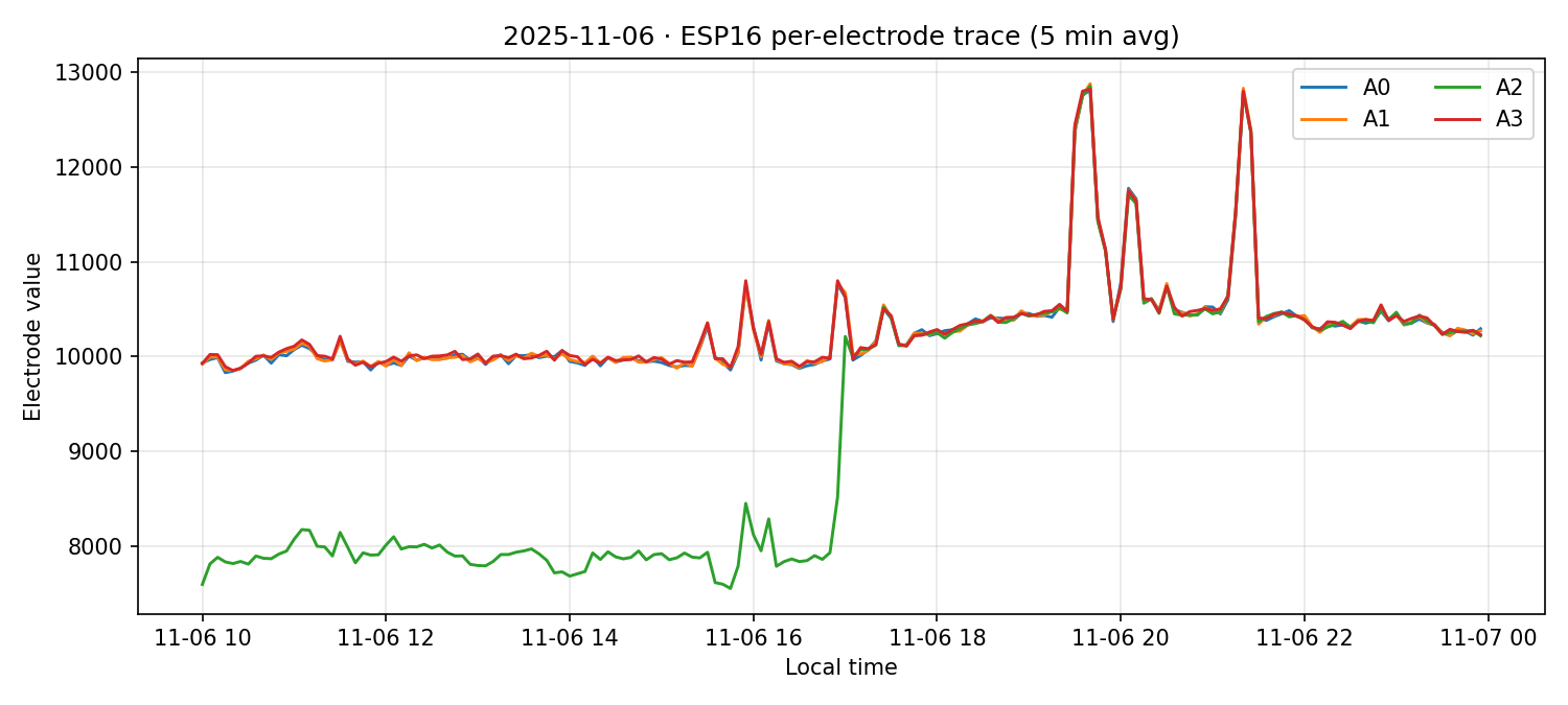
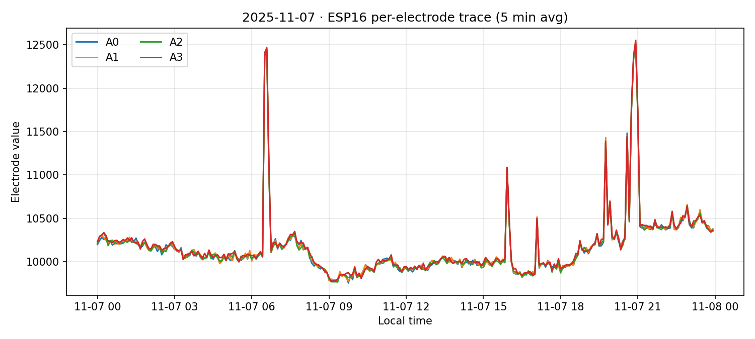
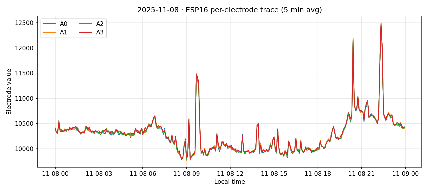
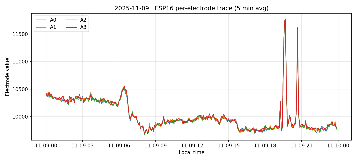
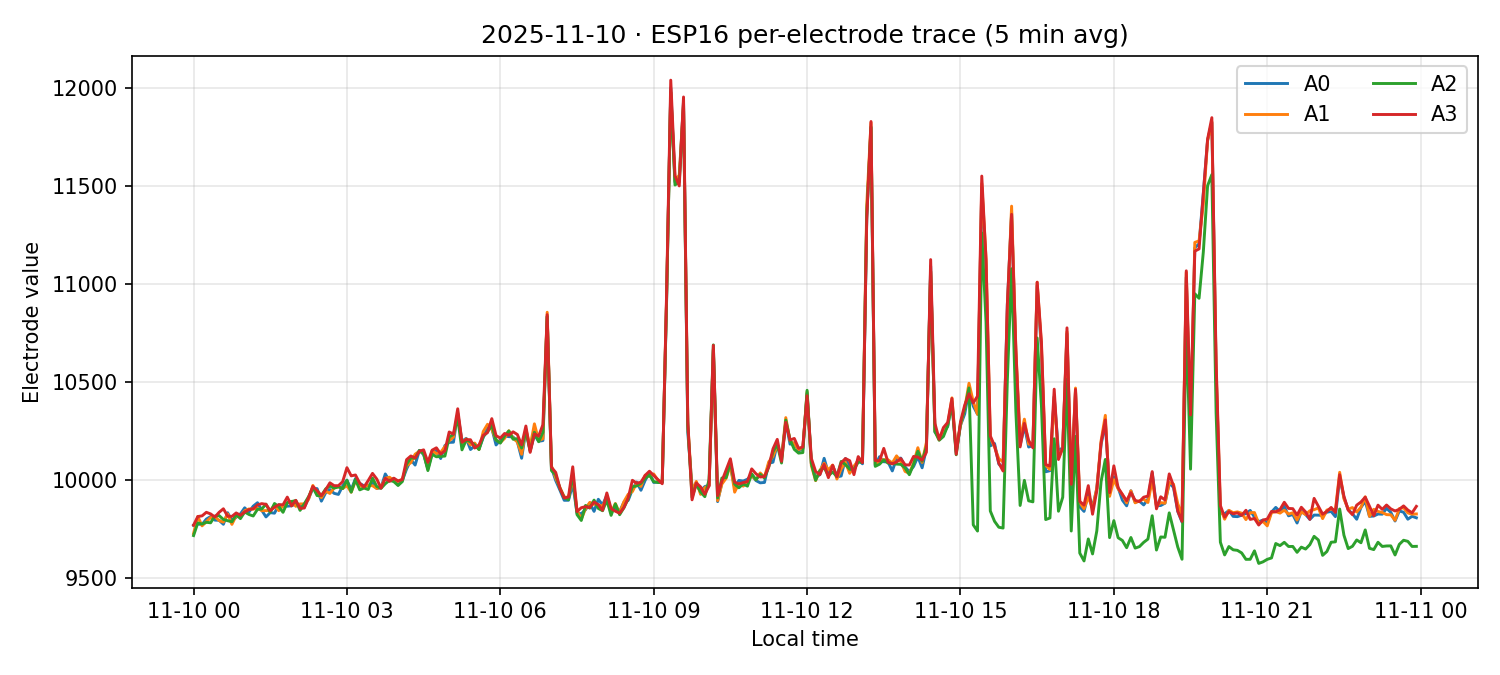
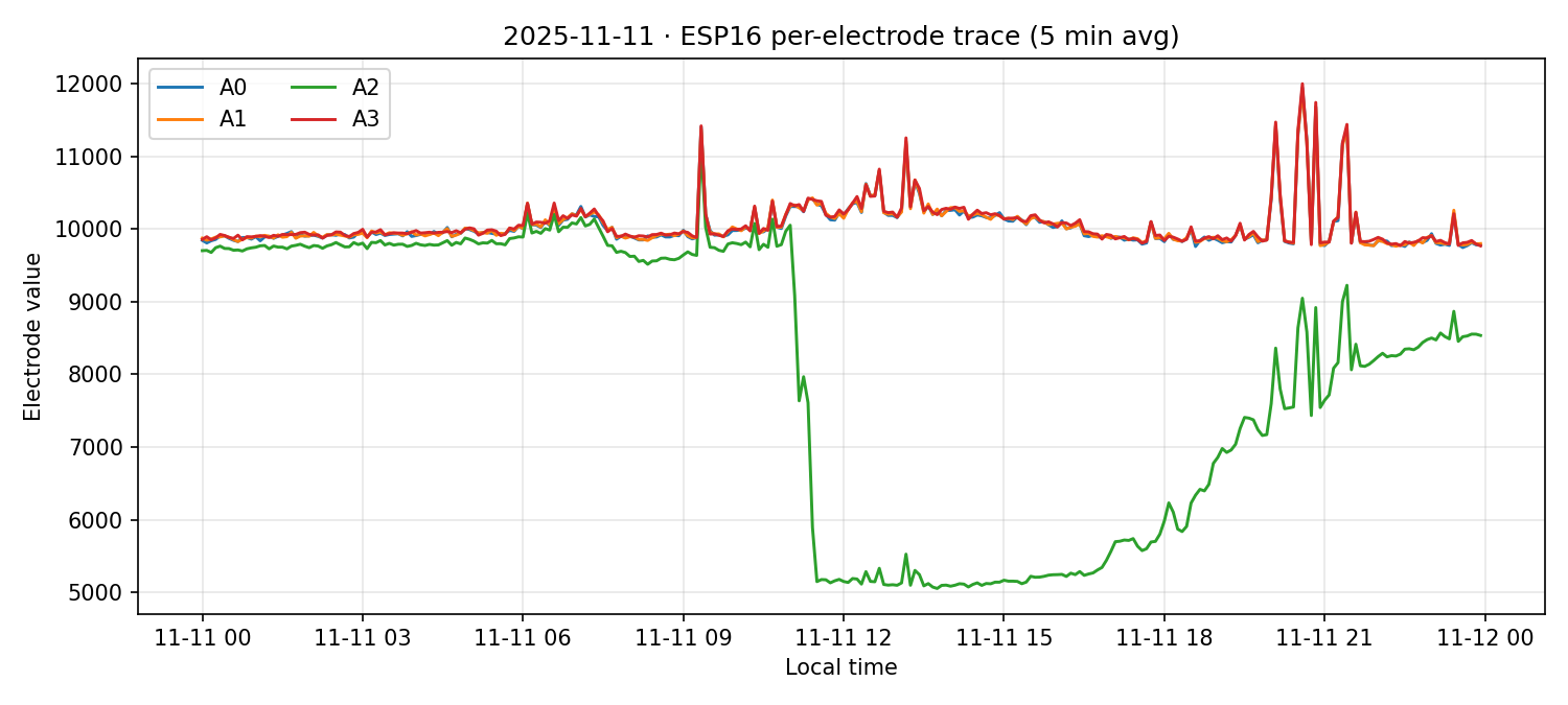
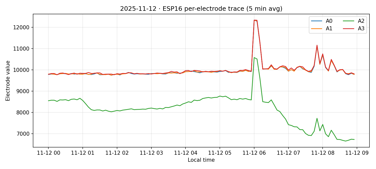
Notable per-electrode behavior (ESP16). Entering the window around 10:00, electrode a2 sits ~2,000 counts below a0/a1/a3 but remains strongly correlated (identical waveform). Near ~17:00 it steps up to match the other three and "moves in lockstep" for the next four days. On 10 Nov, a2 again runs ~1,000 counts lower overall yet spikes to the same peak levels as the others—i.e., compensatory spike amplitude despite a lower offset baseline. This pattern continues into 11 Nov until ~11:00 local, when a2 abruptly drops by ≈4,500 counts, then gradually recovers over ~12 hours to a plateau ≈2,000 counts below the other three—still phase‑locked and waveform‑matched. On 12 Nov it fluctuates and dips again around local noon, remaining coherent in shape even as its baseline shifts.
Three‑Level Hierarchical Model
Level 1: AC coherence defines electrical domains. If electrodes share the same AC rhythm (same phase, same main frequencies), they likely belong to one electrically coherent domain—a functional unity that may represent one organism or a strongly coupled network region. If two electrodes on the same substrate show clearly different AC patterns (different phase, different dominant periods) that persist over time, they likely belong to two weakly coupled or uncoupled domains—separate colonies or regions not yet electrically integrated. In this experiment, Group 1 (ESP05/11/13) and Group 2 (ESP01/08/14/16/17) exhibit distinct diurnal AC patterns, suggesting they represent two semi‑independent electrical domains within the same substrate.
Level 2: DC offset marks local state within a domain. When AC remains locked (same domain) but one electrode's DC baseline drifts away from others for hours or days, this indicates the same global rhythm with a different local operating point. DC offset thus serves as a local state variable within the same electrical domain. The state itself will be characterized later by FFT/PSD profiles (what frequencies are strong), variance patterns, and response characteristics. Examples in this data include ESP16's a2 electrode maintaining phase‑lock while its DC baseline shifts by thousands of counts, and ESP05's transient spread increase where electrodes remain AC‑coherent but DC separation increases.
Level 3: Spikes represent state‑dependent evoked responses. Transient spikes or excursions on top of the DC baseline are evoked responses to stimuli (misting, salt, temperature changes, etc.), not just background rhythm. These responses are state‑dependent: the same stimulus will produce different spike shapes, latencies, and amplitudes depending on the underlying Level‑1/Level‑2 state (domain identity and local operating point). This mirrors how excitable media like brains and hearts are analyzed: background rhythm (AC), baseline/resting potential (DC), and evoked responses (spikes/transients) form a complete framework for understanding the system's behavior.
Data & methods
All calculations reuse the Experiment 001A extraction pipeline:
- Source CSVs:
analysis/fungal_state_mapping/outputs/experiment_001a/CSV/espXX_experiment_001a.csv. - New helper:
analysis/fungal_state_mapping/scripts/generate_experiment_001b_plots.pywrites the hourly summaries (derived/espXX_hourly_cycle_by_electrode.csv), per-day sample counts (daily_counts/espXX_daily_electrode_counts.csv), and all figures underexperiments/experiment-001b/assets/. - Local timezone: America/Costa_Rica (UTC−6), using 5-minute resampling for per-day traces.
Daily coverage tables shown in each panel originate from the corresponding CSV in analysis/fungal_state_mapping/outputs/experiment_001b/daily_counts/.
Addendum 001B-1 — ESP16 extended window
Why this addendum. The official 001A window ends at noon on 12 Nov, but ESP16 continued logging. To better understand the evolving behaviour of electrode a2, we pulled an extended window for ESP16 only (06 Nov 16:01 UTC → 15 Nov 16:01 UTC) and generated per‑day per‑electrode plots.
What we did. We exported esp16_001b1_window.csv from InfluxDB and rendered daily 5‑minute resamples for a0–a3. We also quantified a2’s offset against the mean of (a0,a1,a3), and detected step‑like shifts.
What we found (a2 vs a0/a1/a3). Mean offset by day (counts): 06 Nov ≈ −1055; 07–09 Nov near 0 (lockstep); 10 Nov ≈ −87 (compensatory spikes reach peer peaks); 11 Nov ≈ −2027 with a sharp step at ~11:10 local (min ≈ −5444), then gradual recovery; 12 Nov ≈ −1689 with a noon dip (min ≈ −4253). Detected steps at ~17:00 on 06 Nov, ~11:10/11:30 on 11 Nov, and ~13:40 on 12 Nov.
ESP16 per‑day plots (extended)
ESP16 d23 (extended)
Scripts used. Extraction: analysis/fungal_state_mapping/scripts/extract_experiment_001b1_esp16.py. Plotting & a2 summary: analysis/fungal_state_mapping/scripts/generate_experiment_001b1_esp16.py. Daily traces use the same 5‑minute resampling approach as the original 001B generator.