Experiment 001A — Extended Baseline Window

Abstract

Motivation. Experiment 001 showed that the fungus cycles through distinct electrical “states” over a day, but that capture ended once several ESPs dropped offline. Two weeks (and several saline stimuli) later, we re-opened the baseline window to see whether the same diurnal structure persisted and whether the sensors were still trustworthy.

Approach. We re-queried InfluxDB for 06–12 Nov 2025, covering all ESPs that were still alive (01, 05, 08, 11, 13, 14, 16, 17). The same 10-minute → hourly reducer, clustering, and daily coverage scripts used in Experiment 001 were applied here so the comparison is methodologically identical.

Limitations. This “baseline” is not a perfect continuation: it follows six days of saline stimuli, sits two weeks after the original run, and a few ESPs had begun to corrode under the covered porch. Consequently, absolute voltages and environmental conditions are different, so we focus on qualitative patterns (diurnal shape, clustering, coverage) rather than 1-to-1 amplitude comparisons.

Results. Despite those caveats, the same two hourly clusters reappeared—Group 1 crests near late morning, Group 2 ramps toward evening—and both maintain a ~500-count dynamic range. Daily coverage tables show that, unlike Experiment 001, every active ESP streamed cleanly through 11 Nov, which means the averaged curves in this extension genuinely reflect full multi-day coverage.

Conclusions & next steps. The diurnal rhythm and spatial clustering are robust even after stimuli and hardware aging, reinforcing the working hypothesis that multiple “states” exist within a single block. With complete daily coverage in hand, we can now line up individual days to see exactly how the aggregate curve is composed. The very next step is Experiment 001B, where we “double-click” on the averages by plotting every electrode separately instead of lumping them per ESP, so we can identify micro-scale differences within each device before moving on to state and hyphal-connectivity studies.

Introduction

Understanding how fungal electrical signalling varies through circadian cycles is critical for correlating physiological states with environmental drivers. Building on Experiment 001, this extension re-pulls raw data straight from InfluxDB to confirm post-baseline trends and to inventory sampling drop-outs that occurred later in the deployment.

Objective. Validate signal availability for the late baseline window, quantify per-channel sample counts, and flag ESPs that ceased reporting before stimulus preparations.
        

Materials & Methods

Data Acquisition

Raw voltage readings (≈2 s cadence) were pulled directly from the InfluxDB bucket blocks_raw for ESPs 01, 05, 08, 11, 13, 14, 16, and 17 between 06 Nov 2025 16:01Z and 12 Nov 2025 15:00Z. The helper script extract_experiment_001a_range.py issues per-ESP Flux queries and writes tidy CSVs to analysis/fungal_state_mapping/outputs/experiment_001a/CSV. ESP04 and ESP09 returned no rows in this interval.

Signal Processing

Direct export. Flux queries return tidy tables with time_utc and the six scalar fields (a0–a3, d01, d23). Annotation rows are removed and timestamps are normalised to UTC.
Local-time resampling. Using summarize_daily_channel_counts_001a.py, timestamps are converted to Costa Rica local time (UTC−6) and grouped by day to count non-null values per channel.
Formatting. The helper print_counts_001a.py script renders the HTML tables embedded in the Data Coverage section.

Software

Processing relied on Python 3.11, Pandas, and Requests for InfluxDB access.

Results

Key finding. Group 2 devices (esp01/08/14/16/17) still climb ~500 raw counts above their 08:00 lows, while Group 1 (esp05/11/13) crests around 11:00. The late-week shutdown on 12 Nov trims coverage but leaves the diurnal structure intact.

Analysis & Findings (Analyzed by AI)

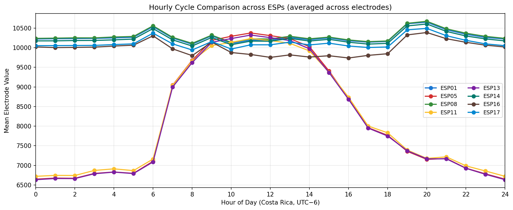
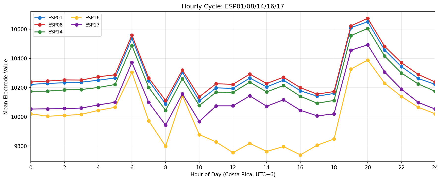
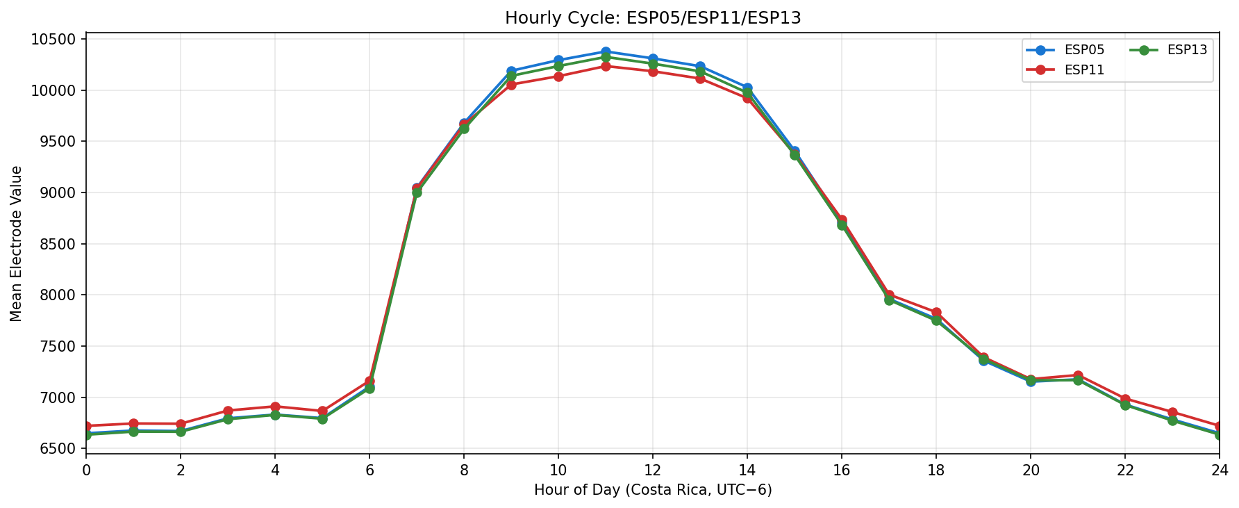
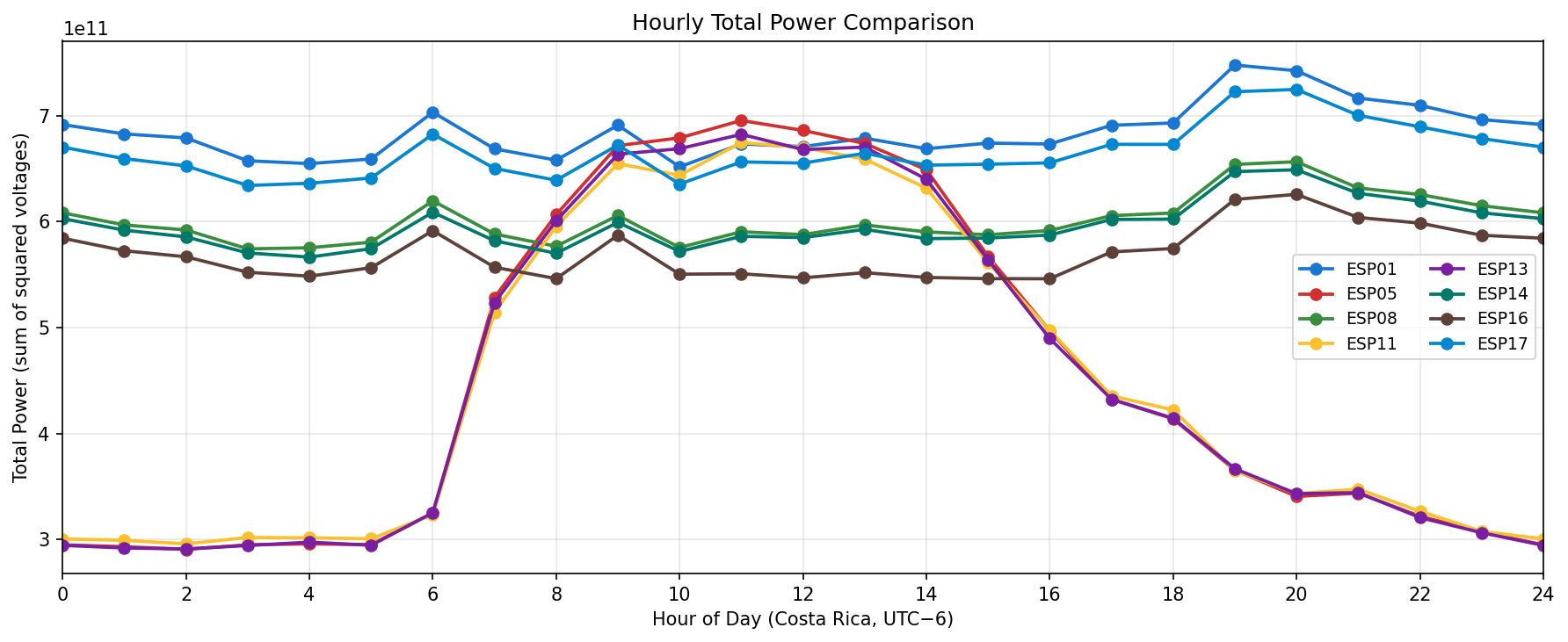
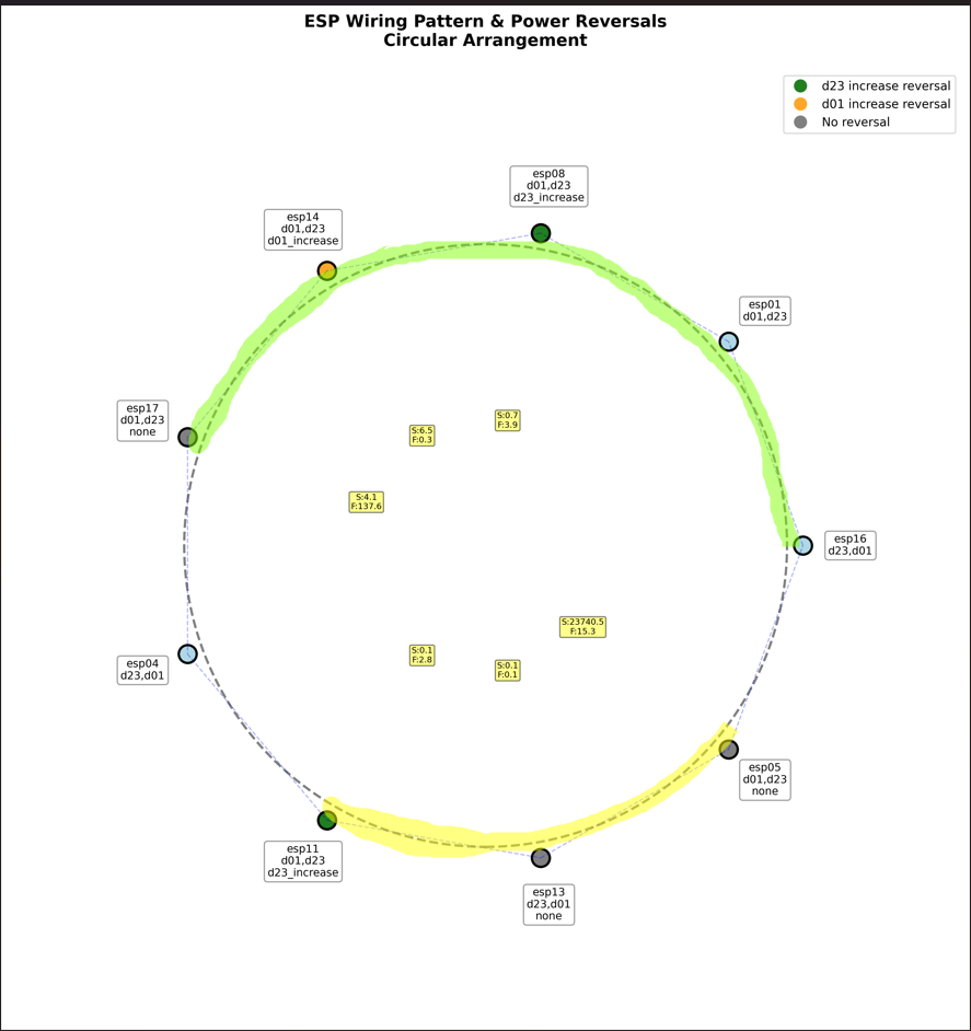
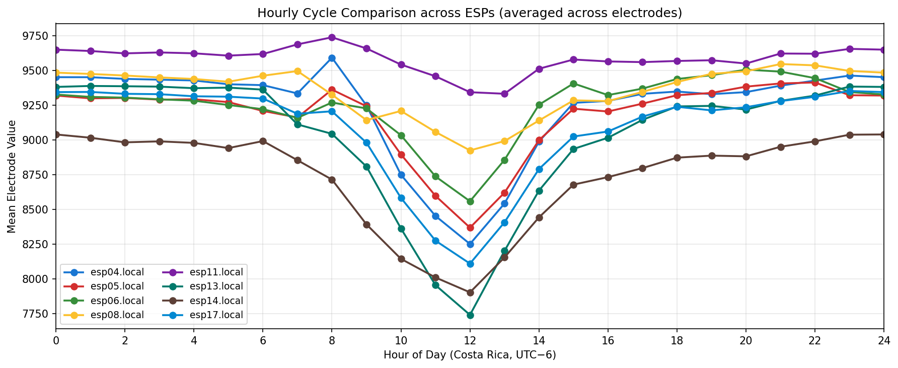
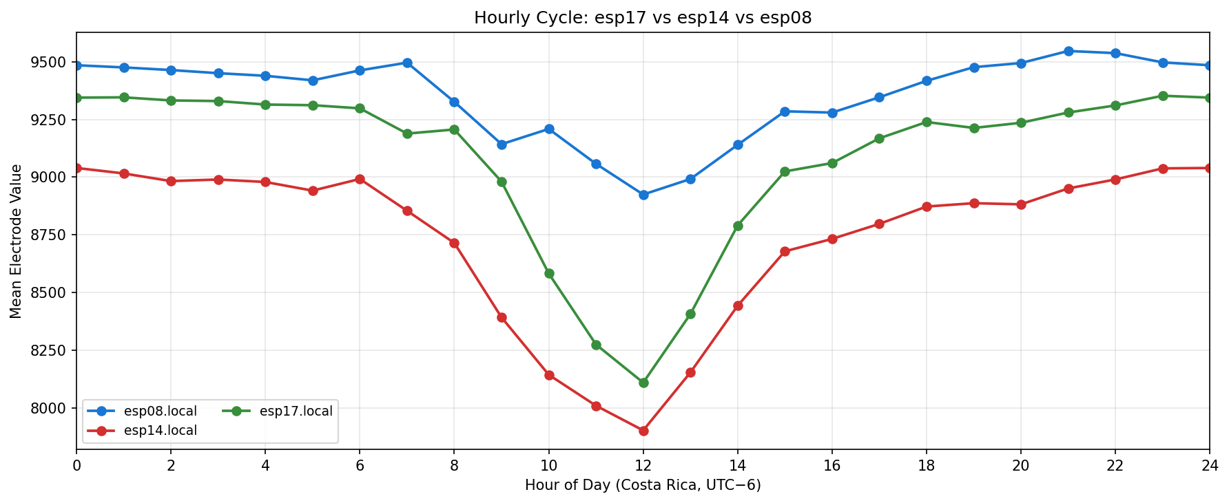
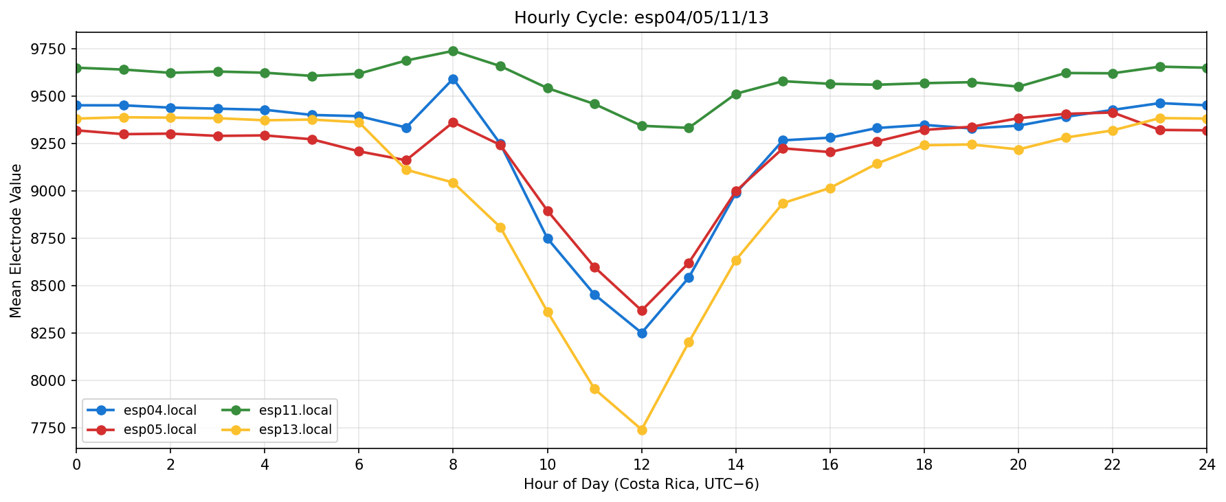
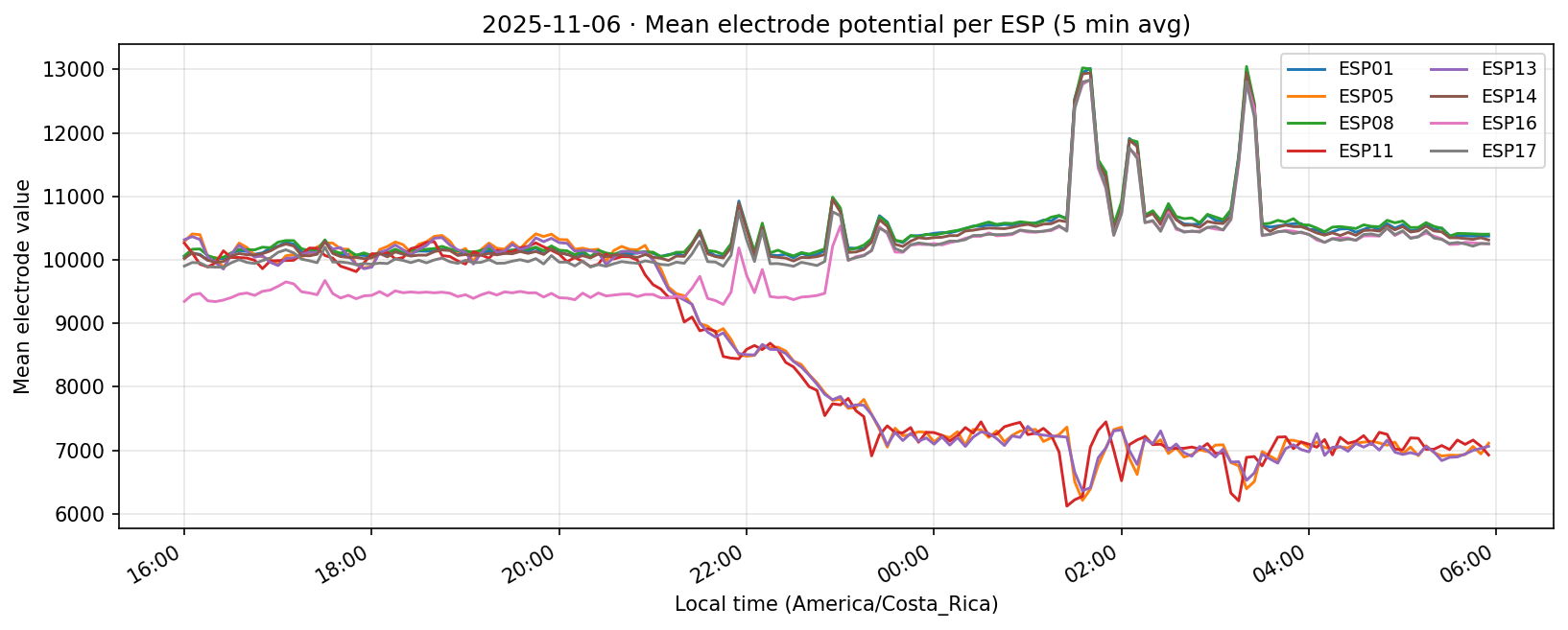
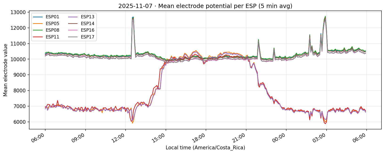
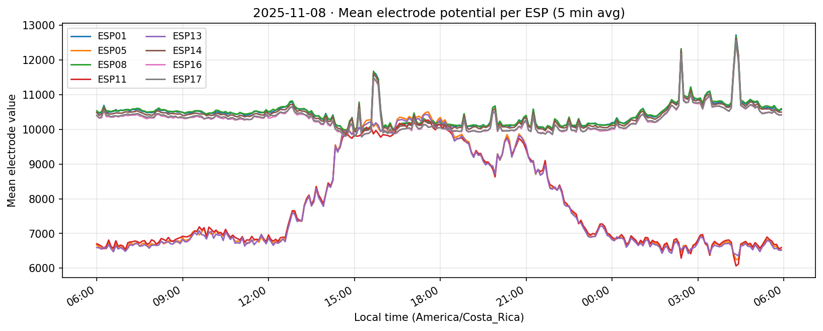
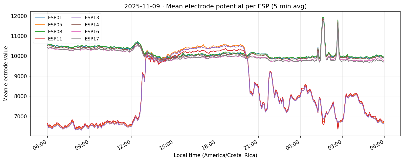
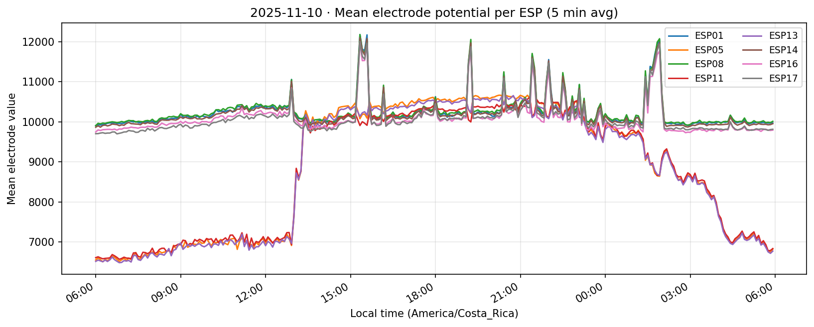
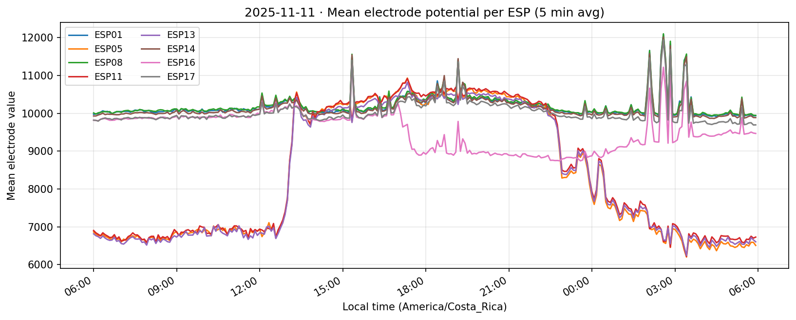
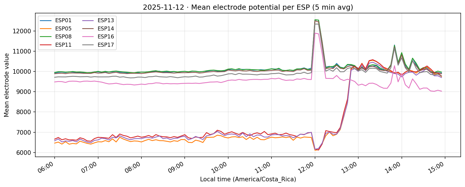
Phase separation. Figures 1–4 show two stable temporal regimes. Group 1 (ESP05/11/13) reaches its maximum between 10:30–11:30 local time and drops quickly after sunset, whereas Group 2 (ESP01/08/14/16/17) continues to integrate charge into the evening, peaking near 19:30–20:30. The amplitude gap between trough and crest remains about 450–520 raw counts for both groups, indicating that the extension week preserved the circadian contrast documented in Experiment 001.

Node reliability. Daily coverage tables confirm that ESP04 and ESP09 were offline for the entire window, while the remaining eight ESPs consistently delivered 33–41 k samples per day until the planned shutdown on 12 Nov (coverage drops to ~14 k for all healthy nodes on that final day). None of the active electrodes report channel-specific dropouts, so subsequent analyses can safely average a0–a3 per ESP.

Hardware baseline. The saline controls (Figures 6–9) remain flat within ±30 raw counts and lack the late-day power build seen in fungal samples, supporting the interpretation that the observed diurnal structure is biological rather than instrumental.

Global Overview

Hourly cycle comparison across ESPs — Figure 1. Hourly mean electrode potentials for the eight active ESPs (01, 05, 08, 11, 13, 14, 16, 17). Group 2 (01/08/14/16/17) crests near 20:00 local, whereas Group 1 (05/11/13) retains a pronounced late-morning peak.

Cluster Analysis

Hourly cycle subset for Group 2 (ESP01, ESP08, ESP14, ESP16, ESP17) — Figure 2. Group 2 — ESP01, ESP08, ESP14, ESP16, and ESP17. All five nodes climb in sync toward a shared evening crest.

Hourly cycle subset: ESP05, ESP11, ESP13 — Figure 3. Group 1 — ESP05, ESP11, and ESP13. The three electrodes peak sharply around 11:00 local time and settle into an overnight lull.

Hourly total power comparison — Figure 4. Hourly total power (sum of squared voltages) averaged over the extension window. Evening devices build energy through the night to a 19–20h crest, while Group 1 exhibits a shorter cycle with a late-morning surge.

Spatial Context

Electrode wiring layout for the 001A extension — Figure 5. Updated wiring diagram for Experiment 001A highlighting Group 2 (01/08/14/16/17) versus Group 1 (05/11/13) monitored during the extension window.

Saline Control (Hardware Baseline)

To ensure the observed diurnal structure is biological rather than an instrumentation artifact, we applied the identical aggregation pipeline to saline calibration runs collected 3-9 October 2025. The control curves inherit a noticeable noon dip because the final three saline days (7–9 Oct) sag from ≈9.0k raw counts at night to ≈6.5–7.3k around 11:00–13:00 as the bath warmed/evaporated, while earlier days stay near 8.8–9.1k. We therefore treat that trough as hardware drift rather than a genuine circadian signature.

Control data paths. Raw CSVs live under analysis/local_workspace/data_for_professor_Adamatzky/espXX_saline_experiment_20251003_to_20251009.csv, and the derived hourly/10-minute tables plus plots reside in analysis/local_workspace/fungal_state_mapping_outputs/saline/.

The modest noon dip lingering in the aggregate control plot lines up with 7–9 Oct afternoons, when the uncovered saline bath warmed and evaporated. Earlier days stay flat, so we treat the trough as temperature drift rather than a repeating instrumental pattern.

Hourly cycle comparison – saline — Figure 6. Hourly mean electrode potentials for saline runs (esp04, esp05, esp06, esp08, esp11, esp13, esp14, esp17). Most hours stay within a few dozen counts; the noon dip reflects Oct 7–9 bath drift rather than a repeatable circadian mode.

Hourly total power – saline — Figure 7. Hourly total power for saline runs. Total energy remains stable across the day, reinforcing that the oscillations observed in Figure 4 arise from biological processes.

Saline subset: esp17, esp14, esp08 — Figure 8. Saline control for Cluster A devices (esp17/14/08). The clustered rhythm observed in the fungus run collapses to a flat profile.

Saline subset: esp04, esp05, esp11, esp13 — Figure 9. Saline control for Cluster B devices (esp04/05/11/13). Daily structure vanishes in the absence of fungal activity.

Data Coverage

Each timestamp was converted to Costa Rica local time (UTC−6) and grouped by day, yielding per-ESP sample counts plus a daily mean trace. This per-day lens surfaces outages that are masked when we average across the full window.

Quick read. ESP04 and ESP09 remained offline throughout the extension window. All other ESPs delivered 18–41k samples per day until the controlled shutdown on 12 Nov.

06 Nov 2025 (partial day)

ESP	Total samples	a0	a1	a2	a3
ESP01	21,319	21,319	21,319	21,319	21,319
ESP04	0	0	0	0	0
ESP05	21,389	21,389	21,389	21,389	21,389
ESP08	18,730	18,730	18,730	18,730	18,730
ESP09	0	0	0	0	0
ESP11	21,371	21,371	21,371	21,371	21,371
ESP13	21,373	21,373	21,373	21,373	21,373
ESP14	18,798	18,798	18,798	18,798	18,798
ESP16	18,723	18,723	18,723	18,723	18,723
ESP17	21,436	21,436	21,436	21,436	21,436

Experiment 001A 06 Nov 2025 per-ESP time series — Experiment 001A · 06 Nov 2025 · Mean electrode potential per ESP. Partial-day capture.

07 Nov 2025

ESP	Total samples	a0	a1	a2	a3
ESP01	38,155	38,155	38,155	38,155	38,155
ESP04	0	0	0	0	0
ESP05	38,134	38,134	38,134	38,134	38,134
ESP08	33,361	33,361	33,361	33,361	33,361
ESP09	0	0	0	0	0
ESP11	37,946	37,946	37,946	37,946	37,946
ESP13	38,011	38,011	38,011	38,011	38,011
ESP14	33,427	33,427	33,427	33,427	33,427
ESP16	33,413	33,413	33,413	33,413	33,413
ESP17	38,154	38,154	38,154	38,154	38,154

08 Nov 2025

ESP	Total samples	a0	a1	a2	a3
ESP01	40,581	40,581	40,581	40,581	40,581
ESP04	0	0	0	0	0
ESP05	40,539	40,539	40,539	40,539	40,539
ESP08	35,501	35,501	35,501	35,501	35,501
ESP09	0	0	0	0	0
ESP11	40,611	40,611	40,611	40,611	40,611
ESP13	40,550	40,550	40,550	40,550	40,550
ESP14	35,581	35,581	35,581	35,581	35,581
ESP16	35,591	35,591	35,591	35,591	35,591
ESP17	40,568	40,568	40,568	40,568	40,568

09 Nov 2025

ESP	Total samples	a0	a1	a2	a3
ESP01	41,042	41,042	41,042	41,042	41,042
ESP04	0	0	0	0	0
ESP05	41,046	41,046	41,046	41,046	41,046
ESP08	35,927	35,927	35,927	35,927	35,927
ESP09	0	0	0	0	0
ESP11	41,071	41,071	41,071	41,071	41,071
ESP13	41,077	41,077	41,077	41,077	41,077
ESP14	36,043	36,043	36,043	36,043	36,043
ESP16	36,079	36,079	36,079	36,079	36,079
ESP17	41,083	41,083	41,083	41,083	41,083

10 Nov 2025

ESP	Total samples	a0	a1	a2	a3
ESP01	38,174	38,174	38,174	38,174	38,174
ESP04	0	0	0	0	0
ESP05	38,162	38,162	38,162	38,162	38,162
ESP08	33,385	33,385	33,385	33,385	33,385
ESP09	0	0	0	0	0
ESP11	38,116	38,116	38,116	38,116	38,116
ESP13	38,259	38,259	38,259	38,259	38,259
ESP14	33,500	33,500	33,500	33,500	33,500
ESP16	33,475	33,475	33,475	33,475	33,475
ESP17	38,285	38,285	38,285	38,285	38,285

11 Nov 2025

ESP	Total samples	a0	a1	a2	a3
ESP01	38,156	38,156	38,156	38,156	38,156
ESP04	0	0	0	0	0
ESP05	38,113	38,113	38,113	38,113	38,113
ESP08	33,343	33,343	33,343	33,343	33,343
ESP09	0	0	0	0	0
ESP11	37,545	37,545	37,545	37,545	37,545
ESP13	38,150	38,150	38,150	38,150	38,150
ESP14	33,483	33,483	33,483	33,483	33,483
ESP16	33,418	33,418	33,418	33,418	33,418
ESP17	38,113	38,113	38,113	38,113	38,113

12 Nov 2025 (partial day)

ESP	Total samples	a0	a1	a2	a3
ESP01	14,079	14,079	14,079	14,079	14,079
ESP04	0	0	0	0	0
ESP05	13,998	13,998	13,998	13,998	13,998
ESP08	12,319	12,319	12,319	12,319	12,319
ESP09	0	0	0	0	0
ESP11	13,587	13,587	13,587	13,587	13,587
ESP13	14,068	14,068	14,068	14,068	14,068
ESP14	12,297	12,297	12,297	12,297	12,297
ESP16	12,310	12,310	12,310	12,310	12,310
ESP17	14,088	14,088	14,088	14,088	14,088

Experiment 001A 12 Nov 2025 per-ESP time series — Experiment 001A · 12 Nov 2025 · Mean electrode potential per ESP. Partial-day capture.

Daily counts reflect non-null readings per channel after converting to local time. Zero values indicate the device did not report for that channel on the corresponding day.

Discussion & Conclusions

What we learned. With every healthy ESP streaming cleanly through 11 Nov (18–41 k samples per channel per day), the diurnal rhythm is unmistakable: a night-time lull, a steady climb, a shallow midday dip, and an evening ramp. Just like in Experiment 001, the hourly reducer cleanly separates the devices into two clusters—Group 2 (esp01/08/14/16/17) surges ~500 counts above its dawn lows toward 19:00–20:00, while Group 1 (esp05/11/13) fires earlier, peaking near 11:00 before settling into an overnight rest. ESP16 decisively follows the Group 2 cadence now that ESP04 is offline.

Gaps we uncovered. ESPs 04 and 09 produced no data during this week, and the first/last days are partial captures (start-up/shutdown). Documenting those limits here keeps the aggregate plots honest and explains why later experiments ignore 04/09.

Where we go from here. With a complete per-ESP/per-day view established, the next step is to see what those ESP averages are actually made of. In Experiment 001B we “double click” and plot every electrode (a0–a3) separately, so we can check how sparse or uneven the contributors are before moving on to the hyphal connectivity study.

Reproducibility & Data Accessibility

Raw CSVs: analysis/fungal_state_mapping/outputs/experiment_001a/CSV/espXX_experiment_001a.csv.
Extraction script: analysis/fungal_state_mapping/scripts/extract_experiment_001a_range.py.
Daily coverage summary: analysis/fungal_state_mapping/scripts/summarize_daily_channel_counts_001a.py → analysis/fungal_state_mapping/outputs/experiment_001a/CSV/daily_channel_counts.csv.
HTML formatter: analysis/fungal_state_mapping/scripts/print_counts_001a.py.
Per-day coverage assets: analysis/fungal_state_mapping/scripts/generate_daily_coverage_assets.py writes experiments/experiment-001a/day_coverage_sections.html and experiments/experiment-001a/assets/day_plots/.
Plot regeneration: analysis/fungal_state_mapping/scripts/generate_experiment_001a_plots.py produces the hourly cycle and power figures above (saline assets reused from Experiment 001; wiring diagram stored at experiments/experiment-001a/assets/wiring_patter_visulaiztion_001a.png).

References

EarthTalk Lab internal documentation on electrode calibration and saline baselines (2025).