Experiment 001 — Diurnal Electrical States

Abstract

Motivation. We suspected the fungus cycles through electrical ΓÇ£statesΓÇ¥ (resting, feeding, growing, etc.) across the day, and that stimuli might trigger different responses depending on the state it is already in. Before naming or modelling those states, we needed to prove they exist and to see how stable the baseline is.

Approach. Using the 24ΓÇô30 Oct 2025 baseline, we averaged raw electrode readings (ESPs 04, 05, 08, 11, 13, 14, 17) into 10-minute blocks, rolled them into hourly means, and clustered the hourly curves. We then applied the exact same reducer to saline-control runs (3ΓÇô9 Oct) to check for hardware artefacts, and finally broke the fungus run back into individual days to see which hours truly contributed to the ΓÇ£average.ΓÇ¥

Results. The fungus traces exhibit a consistent dayΓÇônight rhythm and two spatially coherent clusters. That split raises the possibility that the single physical block may actually host two semi-independent mycelial ΓÇ£organismsΓÇ¥ (or at least two regions connected by too few hyphae to share state quickly). The saline control stayed largely flat, aside from a noon dip on the hottest days that we attribute to bath heating/evaporation rather than instrumentation drift. Daily coverage revealed that only 23ΓÇô25 Oct contained full data, so later hours in the aggregate trace were based on sparse or zero samples.

Conclusions & next steps. The baseline does contain repeatable states, but we need denser data (Experiment 001A) and a temperature-controlled saline repeat before we can label those states or tie stimuli to them. This report documents the processing pipeline, sanity checks, gaps discovered, and the follow-up experiments required.

Introduction

Understanding how fungal electrical signalling varies through circadian cycles is critical for correlating physiological states (“sleeping,” “feeding,” “growing,” etc.) with environmental drivers. We hypothesize that responses are state-dependent—stimulus → state → outcome—so the first question was simply: do repeatable electrical states exist over the day?

Previous EarthTalk experiments highlighted response peaks during stimulus protocols; here we characterize the inherent baseline dynamics. We focus on ESPs encircling a single substrate block, capturing absolute electrode potentials (a0ΓÇôa3) referenced to a shared ground.

To keep the narrative linear, this page follows the same order we worked through in the lab: first the hourly aggregation (Results) to look for states, then a saline sanity check (Saline control) to confirm the rhythm is biological, and finally a per-day coverage audit (Data coverage) that revealed the gaps which triggered Experiment 001A.

Materials & Methods

Data Acquisition

Raw voltage readings were logged every Γëê2 seconds by each electrode channel (a0ΓÇôa3) for ESPs 04, 05, 08, 11, 13, 14, and 17. (ESP07 had already been decommissioned before this baseline run, which is why it does not appear in the figures.) Data were exported to CSV from the InfluxDB bucket blocks_raw using the helper script push_experiment_to_notion.py for esp04 and pre-existing exports for all other ESPs.

Signal Processing

1. Ten-minute block means. For each ESP, samples were partitioned into contiguous 10-minute windows. Within each window, we averaged all readings per electrode, then averaged across a0ΓÇôa3, producing one ΓÇ£mean block potentialΓÇ¥.
2. Hourly aggregation. Ten-minute values whose start time fell within the same clock hour were averaged across the six-day run, yielding a multi-day hourly mean per ESP.
3. State mapping (esp04). Using analyze_fungal_states.py, we computed biological ╧â by subtracting saline noise in quadrature, assigned state bins (S0ΓÇôS4), and produced fixed/rolling baseline visualizations with spike smoothing <3 samples.

Software

Processing relied on Python 3.10+, Pandas, and Matplotlib. Scripts central to this study:

• compute_hourly_cycle_multi_from_csv.py ΓÇö hourly aggregation & plotting from CSV exports.
• compute_means_10min.py ΓÇö 10-minute mean tables, min/max windows, and bin counts.
• analyze_fungal_states.py ΓÇö state classification for targeted windows.

Results

Global Overview

Cluster Analysis

Spatial Context

Saline Control (Hardware Baseline)

To ensure the observed diurnal structure is biological rather than an instrumentation artifact, we applied the identical aggregation pipeline to saline calibration runs collected 3ΓÇô9 October 2025. The aggregate control curve shows a modest noon dip only on the final three days (7ΓÇô9 Oct) when the uncovered bath warmed and partly evaporated; earlier days stay flat within Γëê50 counts. We therefore treat the trough as temperature-driven drift, not a fundamental property of the hardware. Raw saline CSVs live under analysis/local_workspace/data_for_professor_Adamatzky/espXX_saline_experiment_20251003_to_20251009.csv, and the derived hourly tables/plots are in analysis/local_workspace/fungal_state_mapping_outputs/saline/.

Data Coverage

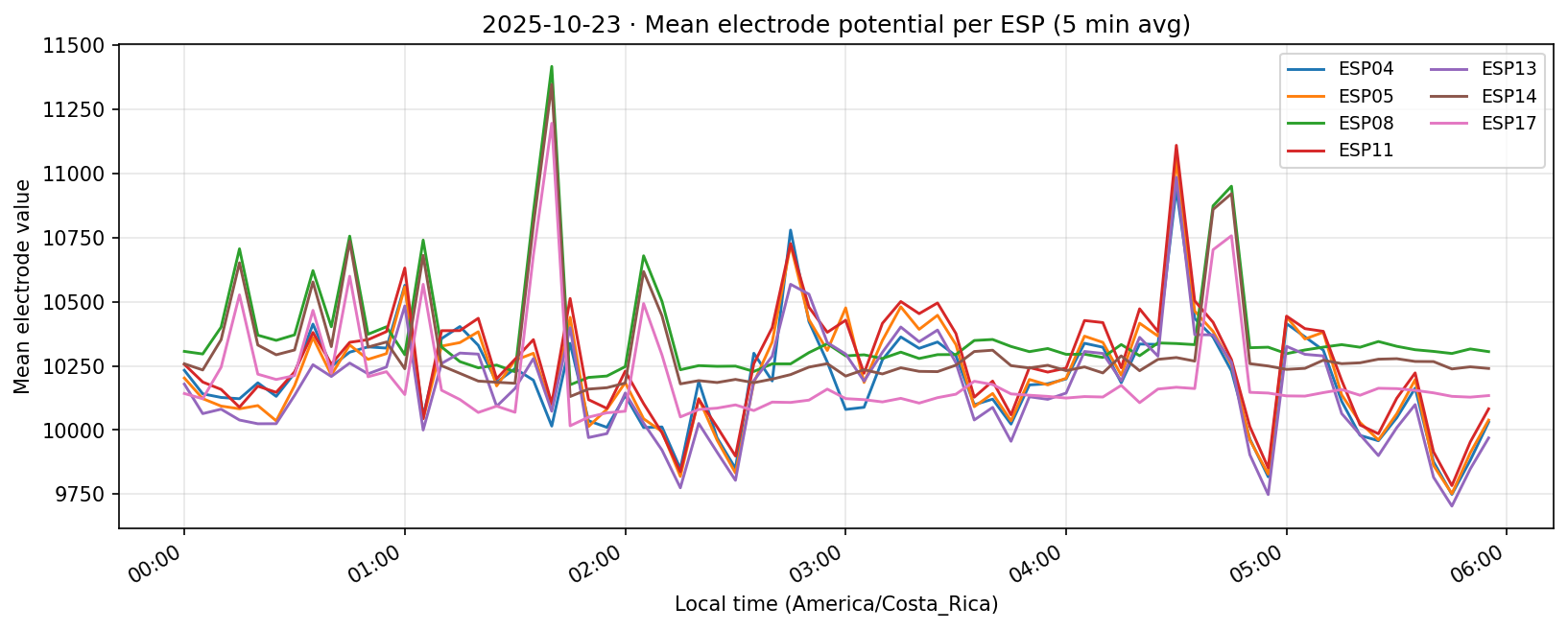
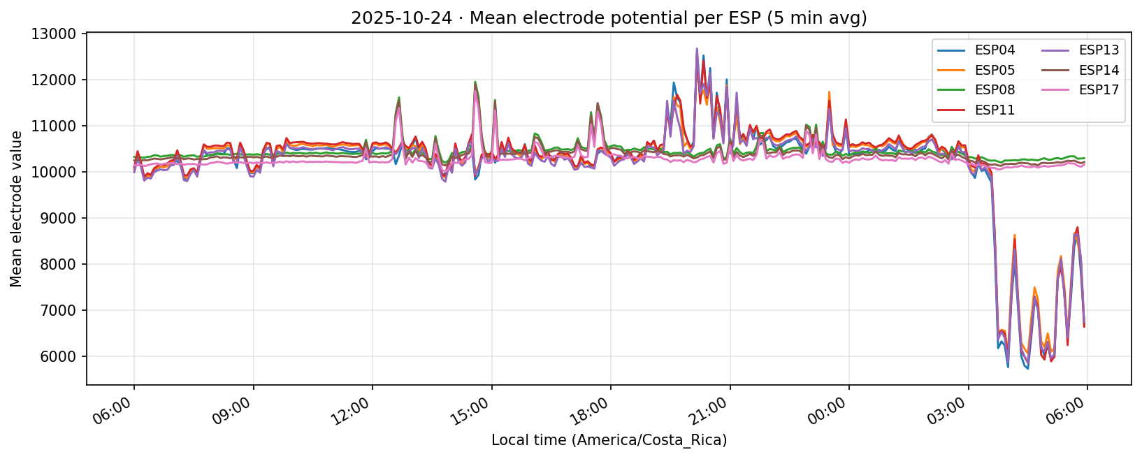
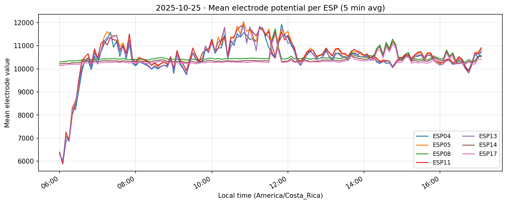
Every timestamp was converted to Costa Rica local time (UTC−6) and grouped by day, yielding per-ESP sample counts and a representative trace for each date. This makes it clear which days actually contribute to the hourly averages.

23 Oct 2025

ESP	Total samples	a0	a1	a2	a3
ESP04	8,536	8,536	8,536	8,536	8,536
ESP05	9,726	9,726	9,726	9,726	9,726
ESP08	8,570	8,570	8,570	8,570	8,570
ESP11	9,718	9,718	9,718	9,718	9,718
ESP13	9,735	9,735	9,735	9,735	9,735
ESP14	8,605	8,605	8,605	8,605	8,605
ESP17	9,706	9,706	9,706	9,706	9,706

24 Oct 2025

ESP	Total samples	a0	a1	a2	a3
ESP04	33,162	33,162	33,162	33,162	33,162
ESP05	37,051	37,051	37,051	37,051	37,051
ESP08	33,196	33,196	33,196	33,196	33,196
ESP11	37,709	37,709	37,709	37,709	37,709
ESP13	37,681	37,681	37,681	37,681	37,681
ESP14	33,316	33,316	33,316	33,316	33,316
ESP17	37,668	37,668	37,668	37,668	37,668

25 Oct 2025

ESP	Total samples	a0	a1	a2	a3
ESP04	21,938	15,431	15,431	15,431	15,431
ESP05	24,890	17,487	17,487	17,487	17,487
ESP08	21,964	15,446	15,446	15,446	15,446
ESP11	24,936	17,533	17,533	17,533	17,533
ESP13	24,988	17,575	17,575	17,575	17,575
ESP14	22,075	15,539	15,539	15,539	15,539
ESP17	24,944	17,556	17,556	17,556	17,556

26 Oct 2025

ESP	Total samples	a0	a1	a2	a3
ESP04	26,886	0	0	0	0
ESP05	30,620	0	0	0	0
ESP08	26,997	0	0	0	0
ESP11	30,579	0	0	0	0
ESP13	30,662	0	0	0	0
ESP14	27,001	0	0	0	0
ESP17	30,640	0	0	0	0

27 Oct 2025

ESP	Total samples	a0	a1	a2	a3
ESP04	0	0	0	0	0
ESP05	37,179	0	0	0	0
ESP08	32,646	0	0	0	0
ESP11	37,007	0	0	0	0
ESP13	37,292	0	0	0	0
ESP14	32,695	0	0	0	0
ESP17	37,255	0	0	0	0

28 Oct 2025

ESP	Total samples	a0	a1	a2	a3
ESP04	0	0	0	0	0
ESP05	37,641	0	0	0	0
ESP08	32,900	0	0	0	0
ESP11	37,580	0	0	0	0
ESP13	37,595	0	0	0	0
ESP14	32,966	0	0	0	0
ESP17	37,578	0	0	0	0

29 Oct 2025

ESP	Total samples	a0	a1	a2	a3
ESP04	0	0	0	0	0
ESP05	37,883	0	0	0	0
ESP08	33,197	0	0	0	0
ESP11	37,717	0	0	0	0
ESP13	37,946	0	0	0	0
ESP14	33,207	0	0	0	0
ESP17	37,918	0	0	0	0

30 Oct 2025

ESP	Total samples	a0	a1	a2	a3
ESP04	0	0	0	0	0
ESP05	28,115	0	0	0	0
ESP08	24,542	0	0	0	0
ESP11	28,174	0	0	0	0
ESP13	28,084	0	0	0	0
ESP14	24,601	0	0	0	0
ESP17	28,098	0	0	0	0

Daily counts reflect non-null readings per channel after converting to Costa Rica local time. Zero values indicate the channel did not report that day.

Discussion & Conclusions

What we learned. The hourly reducer shows that the fungus naturally settles into a night-time lull, climbs through the morning, dips slightly around noon, then ramps again toward evening. Two spatial clusters behave almost like twins, which hints that location (moisture, shade, airflow) influences the baseline voltage.

Why the saline check matters. Running the same math on the saline bath confirmed that the instrumentation itself stays essentially flat; the only wiggle is the noon dip on 7ΓÇô9 Oct when the bath warmed and evaporated. That gives us confidence that the bigger swings in the fungus traces are biological and not an ADC quirk.

Gaps we uncovered. Once we inspected the daily counts we saw that most channels went silent after 25 Oct. Instead of quietly averaging in hours with no true data, we documented the gap here and spun up Experiment 001A to redo the baseline with solid coverage.

Where we go from here. The concrete follow-ups (canonical baseline, saline rerun, hyphal-connectivity test) are listed in the Future Experiments section so they stay visible as active work items.

Future Experiments

• Baseline reboot (Experiment 001A). Use the 06ΓÇô12 Nov capture (all channels healthy) as the canonical baseline going forward, and rerun the hourly clustering on that dataset to confirm the spatial groupings hold when coverage is complete.
• Temperature-controlled saline repeat. Re-run the saline baseline with the bath in a thermostated enclosure (or at least covered and continuously topped off) to confirm that the noon dip truly tracks ambient heating/evaporation. Capturing synchronized ambient temperature alongside the control will let us regress out residual drift and tighten future normalization steps.
• Hyphal connectivity / state-transfer study. Start with a lightly inoculated block, log per-hour states while regions are poorly connected, then let the hyphae knit together and monitor whether the two electrical clusters synchronize. This will tell us whether a minimum hyphal ΓÇ£bandwidthΓÇ¥ is required for full state sharing.

Reproducibility & Data Accessibility

• Raw CSVs: analysis/fungal_state_mapping/outputs/experiment_001/CSV/espXX_experiment_001.csv.
• Extraction script: analysis/fungal_state_mapping/scripts/extract_experiment_001_range.py.
• Hourly aggregation: compute_hourly_cycle_multi_from_csv.py, compute_means_10min.py, analyze_fungal_states.py, query_influx_mean_std.py.
• Daily coverage assets: analysis/fungal_state_mapping/scripts/generate_daily_coverage_assets.py writes experiments/experiment-001/day_coverage_sections.html and experiments/experiment-001/assets/day_plots/.
• Legacy state plots: fixed_baseline_states.png, rolling_baseline_states.png (ESP04 focus).

References

EarthTalk Lab internal documentation on electrode calibration and saline baselines (2025).